Expectation-Maximization (E-M)
- apparently circular logic
- use model to update latent (hidden) variables
- use latent variables to updade model
- iteration maximizes likelihood
- can use momentum for local minima
Clustering
- group similar data points
k-means
- E-M clustering algorithm
- choose a set of anchor points randomly from data
- iteration
- assign data points to the closest anchor
- update anchor to the mean of closest points
- can assess number of clusters by plotting total distance of points to anchors versus their number and look for the "elbow"
Voronoi tesselation
- partition of space closest to anchor points
import matplotlib.pyplot as plt
from scipy.spatial import Voronoi,voronoi_plot_2d
import numpy as np
import time
#
# k-means parameters
#
npts = 1000
nsteps = 1000
momentum = 0.
xs = [0,5,10]
ys = [0,10,5]
np.random.seed(10)
#
# generate random data
#
x = np.array([])
y = np.array([])
for i in range(len(xs)):
    x = np.append(x,np.random.normal(loc=xs[i],scale=1,size=npts))
    y = np.append(y,np.random.normal(loc=ys[i],scale=1,size=npts))

def kmeans(x,y,momentum,nclusters):
    #
    # choose starting points
    #
    indices = np.random.uniform(low=0,high=len(x),size=nclusters).astype(int)
    mux = x[indices]
    muy = y[indices]
    #
    # do k-means iteration
    #
    for i in range(nsteps):
        #
        # find closest points
        #
        X = np.outer(x,np.ones(len(mux)))
        Y = np.outer(y,np.ones(len(muy)))
        Mux = np.outer(np.ones(len(x)),mux)
        Muy = np.outer(np.ones(len(x)),muy)
        distances = np.sqrt((X-Mux)**2+(Y-Muy)**2)
        mins = np.argmin(distances,axis=1)
        #
        # update means
        #
        for i in range(len(mux)):
            index = np.where(mins == i)
            mux[i] = np.sum(x[index])/len(index[0])
            muy[i] = np.sum(y[index])/len(index[0])
    #
    # find distances
    #
    distances = 0
    for i in range(len(mux)):
        index = np.where(mins == i)
        distances += np.sum(np.sqrt((x[index]-mux[i])**2+(y[index]-muy[i])**2))
    return mux,muy,distances

def plot_kmeans(x,y,mux,muy):
    xmin = np.min(x)
    xmax = np.max(x)
    ymin = np.min(y)
    ymax = np.max(y)
    fig,ax = plt.subplots()
    plt.plot(x,y,'.')
    plt.plot(mux,muy,'r.',markersize=20)
    plt.xlim(xmin,xmax)
    plt.ylim(xmin,xmax)
    plt.title(f"{len(mux)} clusters")
    plt.show()

def plot_Voronoi(x,y,mux,muy):
    xmin = np.min(x)
    xmax = np.max(x)
    ymin = np.min(y)
    ymax = np.max(y)
    fig,ax = plt.subplots()
    plt.plot(x,y,'.')
    vor = Voronoi(np.stack((mux,muy),axis=1))
    voronoi_plot_2d(vor,ax=ax,show_points=True,show_vertices=False,point_size=20)
    plt.xlim(xmin,xmax)
    plt.ylim(xmin,xmax)
    plt.title(f"{len(mux)} clusters")
    plt.show()

distances = np.zeros(5)

mux,muy,distances[0] = kmeans(x,y,momentum,1)
plot_kmeans(x,y,mux,muy)

mux,muy,distances[1] = kmeans(x,y,momentum,2)
plot_kmeans(x,y,mux,muy)

mux,muy,distances[2] = kmeans(x,y,momentum,3)
plot_Voronoi(x,y,mux,muy)

mux,muy,distances[3] = kmeans(x,y,momentum,4)
plot_Voronoi(x,y,mux,muy)

mux,muy,distances[4] = kmeans(x,y,momentum,5)
plot_Voronoi(x,y,mux,muy)

fig,ax = plt.subplots()
plt.plot(np.arange(1,6),distances,'o')
plt.xlabel('number of clusters')
plt.ylabel('total distances to clusters')
ax.xaxis.get_major_locator().set_params(integer=True)
plt.show()


issues
- hard boundary can't respond to points just beyond the boundary
- no probability model
Kernel Density Estimation
Gaussian mixture models
- also called kernel density estimation, ...
- soft E-M clustering with Gaussian distributions
- can prune clusters with low probability
In $D$ dimensions a mixture model can be written by factoring the density over multivariate Gaussians, where $c_m$ refers to the $m$th Gaussian with mean $\vec{\mu}_m$ and variance $\vec{\sigma}_m$:
$$ \begin{eqnarray} p(\vec{x}) &=& \sum_{m=1}^M p(\vec{x},c_m) \\ &=& \sum_{m=1}^M p(\vec{x}|c_m)~p(c_m) \\ &=& \sum_{m=1}^M \prod_{d=1}^D \frac{1}{\sqrt{2\pi\sigma_{m,d}^2}} e^{-(x_d-\mu_{m,d})^2/2\sigma_{m,d}^2}~p(c_m) \end{eqnarray} $$
The means are updated with the conditional distribution:
$$ \begin{eqnarray} \vec{\mu}_m &=& \int \vec{x}~p(\vec{x}|c_m)~\vec{dx} \\ &=& \int \vec{x}~\frac{p(c_m|\vec{x})}{p(c_m)} p(\vec{x})~d\vec{x} \\ &\approx& \frac{1}{Np(c_m)} \sum_{n=1}^N \vec{x}_n~p(c_m|\vec{x}_n) \end{eqnarray} $$
The variances are updated with the conditional distribution:
$$ {\sigma}_{m,d} \approx \frac{1}{Np(c_m)} \sum_{n=1}^N (x_{n,d}-\vec{\mu}_{m,d})^2~p(c_m|x_{n,d}) ~~~~, $$
The expansion weights are updated with the conditional distribution:
$$ \begin{eqnarray} p(c_m) &=& \int_{-\infty}^\infty p(\vec{x},c_m)~d\vec{x} \\ &=& \int_{-\infty}^\infty p(c_m|\vec{x})~p(\vec{x})~d\vec{x} \\\ &\approx& \frac{1}{N} \sum_{n=1}^N p(c_m|\vec{x}_n) ~~~~. \end{eqnarray} $$
The conditional distribution is then updated with the means, variances, and weights, completing one E-M setp:
$$ \begin{eqnarray} p(c_m|\vec{x}) &=& \frac{p(\vec{x},c_m)}{p(\vec{x})} \\ &=& \frac{p(\vec{x}|c_m)~p(c_m)}{\sum_{m=1}^M p(\vec{x}|c_m)~p(c_m)} \end{eqnarray} $$
import matplotlib.pyplot as plt
from scipy.spatial import Voronoi,voronoi_plot_2d
import numpy as np
import time
#
# Gaussuam mixture model parameters
#
npts = 3000
nclusters = 3
nsteps = 25
nplot = 100
xs = [0,5,10]
ys = [0,10,5]
np.random.seed(0)
#
# generate random data
#
x = np.array([])
y = np.array([])
for i in range(len(xs)):
    x = np.append(x,np.random.normal(loc=xs[i],scale=1,size=npts//nclusters))
    y = np.append(y,np.random.normal(loc=ys[i],scale=1,size=npts//nclusters))
#
# choose starting points and initialize
#
indices = np.random.uniform(low=0,high=len(x),size=nclusters).astype(int)
mux = x[indices]
muy = y[indices]
varx = (np.max(x)-np.min(x))**2
vary = (np.max(y)-np.min(y))**2
pc = np.ones(nclusters)/nclusters
#
# plot before iteration
#
fig,ax = plt.subplots()
plt.plot(x,y,'.')
plt.errorbar(mux,muy,xerr=np.sqrt(varx),yerr=np.sqrt(vary),fmt='r.',markersize=20)
plt.autoscale()
plt.title('before iteration')
plt.show()
#
# do E-M iterations
#
for i in range(nsteps):
    #
    # construct matrices
    #
    xm = np.outer(x,np.ones(nclusters))
    ym = np.outer(y,np.ones(nclusters))
    muxm = np.outer(np.ones(npts),mux)
    muym = np.outer(np.ones(npts),muy)
    varxm = np.outer(np.ones(npts),varx)
    varym = np.outer(np.ones(npts),varx)
    pcm = np.outer(np.ones(npts),pc)
    #
    # use model to update probabilities
    #
    pvgc = (1/np.sqrt(2*np.pi*varxm))*\
       np.exp(-(xm-muxm)**2/(2*varxm))*\
       (1/np.sqrt(2*np.pi*varym))*\
       np.exp(-(ym-muym)**2/(2*varym))
    pvc = pvgc*np.outer(np.ones(npts),pc)
    pcgv = pvc/np.outer(np.sum(pvc,1),np.ones(nclusters))
    #
    # use probabilities to update model
    #
    pc = np.sum(pcgv,0)/npts
    mux = np.sum(xm*pcgv,0)/(npts*pc)
    muy = np.sum(ym*pcgv,0)/(npts*pc)
    varx = 0.1+np.sum((xm-muxm)**2*pcgv,0)/(npts*pc)
    vary = 0.1+np.sum((ym-muym)**2*pcgv,0)/(npts*pc)
#
# plot after iteration
#
fig,ax = plt.subplots()
plt.plot(x,y,'.')
plt.errorbar(mux,muy,xerr=np.sqrt(varx),yerr=np.sqrt(vary),fmt='r.',markersize=20)
plt.autoscale()
plt.title('after iteration')
plt.show()
#
# plot distribution
#
xplot = np.linspace(np.min(x),np.max(x),nplot)
yplot = np.linspace(np.min(y),np.max(y),nplot)
(X,Y) = np.meshgrid(xplot,yplot)
p = np.zeros((nplot,nplot))
for c in range(nclusters):
    p += np.exp(-(X-mux[c])**2/(2*varx[c]))/np.sqrt(2*np.pi*varx[c])\
       *np.exp(-(Y-muy[c])**2/(2*vary[c]))/np.sqrt(2*np.pi*vary[c])\
       *pc[c]
fig, ax = plt.subplots(subplot_kw={"projection":"3d"})
ax.plot_surface(X,Y,p)
plt.title('probability distribution')
plt.show()


issues
- difficult to represent uniform or smooth distributions
- can't include priors on the distribution
Cluster-Weighted Modeling
- also called mixture of experts, Bayesian networks, ...
- put functional models in Gaussian kernels
- can use covariances in low dimensions, variances in high dimensions
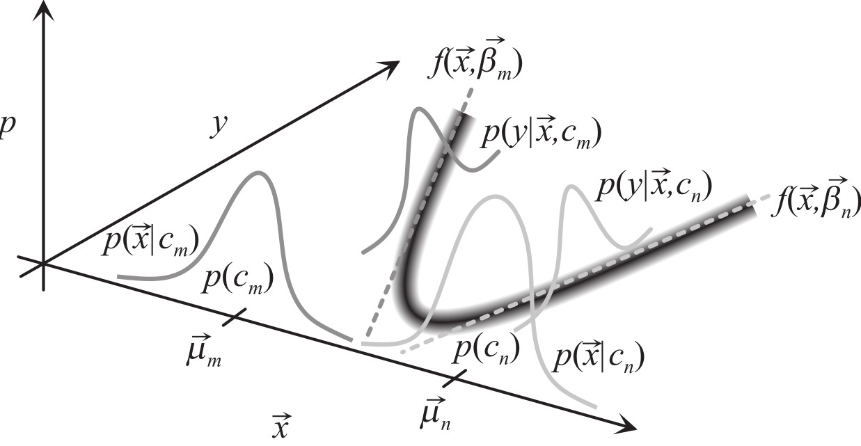
Expand the density in clusters that contain three terms: a weight $p(c_m)$, a domain of influence in the input space $p(\vec x|c_m)$, and a dependence in the output space $p(y|\vec{x},c_m)$:
$$ \begin{eqnarray} p(y,{\vec x}) &=& \sum_{m=1}^M p(y,{\vec x},c_m) \\ &=& \sum_{m=1}^M p(y,{\vec x}|c_m)~p(c_m) \\ &=& \sum_{m=1}^M p(y|{\vec x},c_m)~p({\vec x}|c_m)~p(c_m) \end{eqnarray} $$
The mean of the Gaussian is now a function $f$ that depends on $\vec{x}$ and a set of parameters $\vec{\beta}_m$:
$$ \begin{eqnarray} p(y|{\vec x},c_m) = \frac{1}{\sqrt{2\pi\sigma_{m,y}^2}} e^{-[y-f({\vec x},\vec\beta_m)]^2/2\sigma_{m,y}^2} \end{eqnarray} $$
The conditional forecast is:
$$ \begin{eqnarray} \langle y|{\vec x} \rangle &=& \int y~p(y|{\vec x})~dy \\ &=& \int y~\frac{p(y,{\vec x})}{p({\vec x})}~dy \\ &=& \frac{\sum_{m=1}^M \int y~p(y|{\vec x},c_m)~dy~p({\vec x}|c_m)~p(c_m)} {\sum_{m=1}^M p({\vec x}|c_m)~p(c_m)} \\ &=& \frac{\sum_{m=1}^M f({\vec x},{\vec\beta}_m)~p({\vec x}|c_m)~p(c_m)} {\sum_{m=1}^M p({\vec x}|c_m)~p(c_m)} \end{eqnarray} $$
The error in the forecast is:
$$ \begin{eqnarray} \langle \sigma_y^2|{\vec x} \rangle &=& \int (y-\langle y|{\vec x} \rangle)^2 ~ p(y|{\vec x}) ~ dy \\ &=& \int (y^2-\langle y|{\vec x} \rangle^2) ~ p(y|{\vec x}) ~ dy \\ &=& \frac{\sum_{m=1}^M [\sigma_{m,y}^2 + f({\vec x},{\vec\beta}_m)^2]~ p({\vec x}|c_m)~p(c_m)}{\sum_{m=1}^M p({\vec x}|c_m)~p(c_m)} - \langle y | {\vec x} \rangle^2 \end{eqnarray} $$
If we choose a local model that has linear coefficients, $$ f({\vec x},\vec{\beta}_m) = \sum_{i=1}^I \beta_{m,i} f_i({\vec x}) ~~~~, $$ the $j$th coefficient is updated with: $$ \begin{eqnarray} 0 &=& \langle [y-f({\vec x},{\vec\beta}_m)] f_j({\vec x}) \rangle_m \\ &=& \underbrace{\langle yf_j({\vec x}) \rangle_m}_{\displaystyle a_j} - \sum_{i=1}^I \beta_{m,i}~ \underbrace{\langle f_j({\vec x})f_i({\vec x})\rangle_m}_{\displaystyle B_{ji}} \\ \Rightarrow \vec{\beta}_m &=& B^{-1}\cdot{\vec a} \end{eqnarray} $$
modeling states
- cluster function is a table of state probabilities
import matplotlib.pyplot as plt
import numpy as np
#
# state cluster-weighted modeling parameters
#
dim = 2
nstates = 2
nclusters = 5
nsamples = 100
momentum = 0.9
rate = 0.1
min_var = 0.1
niterations = 100
np.random.seed(10)
#
# generate data
#
def translate(dx,dy,a):
   return(np.array((a[0,:]+dx,a[1,:]+dy)))
def scale(sx,sy):
   return(np.array(([sx,0],[0,sy])))
def rotate(theta):
   theta = np.pi*theta/180
   return(np.array(([np.cos(theta),-np.sin(theta)],[np.sin(theta),np.cos(theta)])))
zero_states = scale(3,1)@np.random.randn(dim,nsamples)
zero_states = np.hstack((zero_states,
   translate(20,0,rotate(90)@scale(3,1)@np.random.randn(dim,nsamples))))
nzeros = zero_states.shape[1]
one_states = translate(5,-10,rotate(45)@scale(5,1)@np.random.randn(dim,nsamples))
one_states = np.hstack((one_states,
   translate(5,10,rotate(-45)@scale(5,1)@np.random.randn(dim,nsamples))))
one_states = np.hstack((one_states,
   translate(11,0,rotate(90)@scale(4,1)@np.random.randn(dim,nsamples))))
nones = one_states.shape[1]
points = np.hstack((zero_states,one_states))
states = np.append(np.zeros(nzeros,dtype=int),np.ones(nones,dtype=int))
npts = len(states)
#
# initialize arrays
#
indices = np.random.randint(0,npts,nclusters)
means = points[:,indices]
dmean = np.zeros((dim,nclusters))
variances = np.outer(np.var(points,axis=1),np.ones(nclusters))
pc = np.ones(nclusters)/nclusters # p(c)
pxgc = np.zeros((nclusters,npts)) # p(x|c)
psgxc = np.ones((nclusters,nstates))/nstates # p(s|xc)
#
# plot data
#
plt.plot(zero_states[0,:],zero_states[1,:],ls='',marker='$0$',markeredgecolor='green')
plt.plot(one_states[0,:],one_states[1,:],ls='',marker='$1$',markeredgecolor='orange')
plt.xlim([-10,30])
plt.ylim([-20,20])
#
# plot clusters
#
def plot_var():
   for cluster in range(means.shape[1]):
      x = means[0,cluster]
      y = means[1,cluster]
      type = np.argmax(psgxc[cluster,:])
      dx = np.sqrt(variances[0,cluster])
      dy = np.sqrt(variances[1,cluster])
      plt.plot([x-dx,x+dx],[y,y],'k')
      plt.plot([x,x],[y-dy,y+dy],'k')
      plt.plot([x],[y],'k',marker=f'${type}$',markersize=15)
plot_var()
plt.title('variance clusters before iteration')
plt.show()
#
# do E-M iteration
#
for i in range(niterations):
   for cluster in range(nclusters):
      mean = np.outer(means[:,cluster],np.ones(npts))
      variance = np.outer(variances[:,cluster],np.ones(npts))
      pxgc[cluster,:] = np.prod(np.exp(-(points-mean)**2/(2*variance))\
         /np.sqrt(2*np.pi*variance),0)
   pxc = pxgc*np.outer(pc,np.ones(npts))
   pcgx = pxc/np.outer(np.ones(nclusters),np.sum(pxc,0))
   psxc = psgxc[:,states]*pxc
   pcgsx = psxc/np.outer(np.ones(nclusters),np.sum(psxc,0))
   pc = np.sum(pcgsx,1)/npts
   for cluster in range(nclusters):
      newmean = momentum*dmean[:,cluster]\
         +np.sum(points*np.outer(np.ones(dim),pcgsx[cluster,:]),1)\
         /np.sum(np.outer(np.ones(dim),pcgsx[cluster,:]),1)
      dmean[:,cluster] = newmean-means[:,cluster]
      means[:,cluster] += rate*dmean[:,cluster]
      m = np.outer(means[:,cluster],np.ones(npts))
      variances[:,cluster] = np.sum((points-m)**2\
          *np.outer(np.ones(dim),pcgsx[cluster,:]),1)\
         /np.sum(np.outer(np.ones(dim),pcgsx[cluster,:]),1)\
         +min_var
   for state in range(nstates):
      index = np.argwhere(states == state)
      psgxc[:,state] = np.sum(pcgsx[:,index],1)[:,0]/np.sum(pcgsx[:,:],1)
#
# plot data
#
plt.plot(zero_states[0,:],zero_states[1,:],ls='',marker='$0$',markeredgecolor='green')
plt.plot(one_states[0,:],one_states[1,:],ls='',marker='$1$',markeredgecolor='orange')
plt.xlim([-10,30])
plt.ylim([-20,20])
#
# plot clusters
#
plot_var()
#
# plot decision boundaries
#
ngrid = 100
xmin = np.min(points[0,:])
xmax = np.max(points[0,:])
ymin = np.min(points[1,:])
ymax = np.max(points[1,:])
x = np.linspace(xmin,xmax,ngrid)
y = np.linspace(ymin,ymax,ngrid)
mx,my = np.meshgrid(x,y)
x = np.reshape(mx,(ngrid*ngrid))
y = np.reshape(my,(ngrid*ngrid))
plotpoints = np.vstack((x,y))
pxgc = np.zeros((nclusters,ngrid*ngrid))
for cluster in range(nclusters):
   mean = np.outer(means[:,cluster],np.ones(ngrid*ngrid))
   variance = np.outer(variances[:,cluster],np.ones(ngrid*ngrid))
   pxgc[cluster,:] = np.prod(np.exp(-(plotpoints-mean)**2/(2*variance))\
      /np.sqrt(2*np.pi*variance),0)
pxc = pxgc*np.outer(pc,np.ones(ngrid*ngrid))
p = np.sum(np.outer(psgxc[:,0],np.ones(ngrid*ngrid))*pxc,0)/np.sum(pxc,0)
p = np.reshape(p,(ngrid,ngrid))
plt.contour(mx,my,p,[0.5])
plt.title('variance clusters and decision boundaries after iteration')
plt.show()
#
# plot probability surface
#
fig, ax = plt.subplots(subplot_kw={"projection":"3d"})
ax.plot_wireframe(mx,my,p,rstride=10,cstride=10,color='gray')
plt.plot(zero_states[0,:],zero_states[1,:],zdir='z',ls='',marker='r$0$',markeredgecolor='green')
plt.plot(one_states[0,:],one_states[1,:],zdir='z',ls='',marker='$1$',markeredgecolor='orange')
plt.title('probability of state 0')
plt.show()


import matplotlib.pyplot as plt
import numpy as np
#
# state cluster-weighted modeling parameters
#
dim = 2
nstates = 2
nclusters = 5
nsamples = 100
momentum = 0.9
rate = 0.1
min_var = 0.1
niterations = 100
np.random.seed(10)
#
# generate data
#
def translate(dx,dy,a):
   return(np.array((a[0,:]+dx,a[1,:]+dy)))
def scale(sx,sy):
   return(np.array(([sx,0],[0,sy])))
def rotate(theta):
   theta = np.pi*theta/180
   return(np.array(([np.cos(theta),-np.sin(theta)],[np.sin(theta),np.cos(theta)])))
zero_states = scale(3,1)@np.random.randn(dim,nsamples)
zero_states = np.hstack((zero_states,
   translate(20,0,rotate(90)@scale(3,1)@np.random.randn(dim,nsamples))))
nzeros = zero_states.shape[1]
one_states = translate(5,-10,rotate(45)@scale(5,1)@np.random.randn(dim,nsamples))
one_states = np.hstack((one_states,
   translate(5,10,rotate(-45)@scale(5,1)@np.random.randn(dim,nsamples))))
one_states = np.hstack((one_states,
   translate(11,0,rotate(90)@scale(4,1)@np.random.randn(dim,nsamples))))
nones = one_states.shape[1]
points = np.hstack((zero_states,one_states))
states = np.append(np.zeros(nzeros,dtype=int),np.ones(nones,dtype=int))
npts = len(states)
#
# initialize arrays
#
indices = np.random.randint(0,npts,nclusters)
means = points[:,indices]
dmean = np.zeros((dim,nclusters))
covariances = np.zeros((nclusters,2,2))
covariances[:,0,0] = np.var(points[0,:])
covariances[:,1,1] = np.var(points[1,:])
pc = np.ones(nclusters)/nclusters # p(c)
pxgc = np.zeros((nclusters,npts)) # p(x|c)
psgxc = np.ones((nclusters,nstates))/nstates # p(s|xc)
#
# plot data
#
plt.plot(zero_states[0,:],zero_states[1,:],ls='',marker='$0$',markeredgecolor='green')
plt.plot(one_states[0,:],one_states[1,:],ls='',marker='$1$',markeredgecolor='orange')
plt.xlim([-10,30])
plt.ylim([-20,20])
#
# plot clusters
#
def plot_covar():
   for cluster in range(means.shape[1]):
      x = means[0,cluster]
      y = means[1,cluster]
      type = np.argmax(psgxc[cluster,:])
      w,v = np.linalg.eig(covariances[cluster])
      w = np.sqrt(w)
      plt.plot([x-w[0]*v[0,0],x+w[0]*v[0,0]],[y-w[0]*v[1,0],y+w[0]*v[1,0]],'k')
      plt.plot([x-w[1]*v[0,1],x+w[1]*v[0,1]],[y-w[1]*v[1,1],y+w[1]*v[1,1]],'k')
      plt.plot([x],[y],'k',marker=f'${type}$',markersize=15)
plot_covar()
plt.title('covariance clusters before iteration')
plt.show()
#
# do E-M iteration
#
for i in range(niterations):
   for cluster in range(nclusters):
      mean = np.outer(means[:,cluster],np.ones(npts))
      cinv = np.linalg.pinv(covariances[cluster])
      pxgc[cluster,:] = (np.sqrt(np.linalg.det(cinv))/(2*np.pi)**(dim/2))\
         *np.exp(-np.sum((points-mean)*(cinv@(points-mean)),0)/2)
   pxc = pxgc*np.outer(pc,np.ones(npts))
   pcgx = pxc/np.outer(np.ones(nclusters),np.sum(pxc,0))
   psxc = psgxc[:,states]*pxc
   pcgsx = psxc/np.outer(np.ones(nclusters),np.sum(psxc,0))
   pc = np.sum(pcgsx,1)/npts
   for cluster in range(nclusters):
      newmean = momentum*dmean[:,cluster]\
         +np.sum(points*np.outer(np.ones(dim),pcgsx[cluster,:]),1)\
         /np.sum(np.outer(np.ones(dim),pcgsx[cluster,:]),1)
      dmean[:,cluster] = newmean-means[:,cluster]
      means[:,cluster] += rate*dmean[:,cluster]
      m = np.outer(means[:,cluster],np.ones(npts))
      for d in range(dim):
         covariances[cluster][:,d] = np.sum(np.outer(\
            np.ones(dim),points[d,:]-m[d,:])*(points-m)*\
            np.outer(np.ones(dim),pcgsx[cluster,:]),1)\
            /np.sum(np.outer(np.ones(dim),pcgsx[cluster,:]),1)\
            +min_var
   for state in range(nstates):
      index = np.argwhere(states == state)
      psgxc[:,state] = np.sum(pcgsx[:,index],1)[:,0]/np.sum(pcgsx[:,:],1)
#
# plot data
#
plt.plot(zero_states[0,:],zero_states[1,:],ls='',marker='$0$',markeredgecolor='green')
plt.plot(one_states[0,:],one_states[1,:],ls='',marker='$1$',markeredgecolor='orange')
plt.xlim([-10,30])
plt.ylim([-20,20])
#
# plot clusters
#
plot_covar()
#
# plot decision boundary
#
ngrid = 100
xmin = np.min(points[0,:])
xmax = np.max(points[0,:])
ymin = np.min(points[1,:])
ymax = np.max(points[1,:])
x = np.linspace(xmin,xmax,ngrid)
y = np.linspace(ymin,ymax,ngrid)
mx,my = np.meshgrid(x,y)
x = np.reshape(mx,(ngrid*ngrid))
y = np.reshape(my,(ngrid*ngrid))
plotpoints = np.vstack((x,y))
pxgc = np.zeros((nclusters,ngrid*ngrid))
for cluster in range(nclusters):
   mean = np.outer(means[:,cluster],np.ones(ngrid*ngrid))
   cinv = np.linalg.pinv(covariances[cluster])
   pxgc[cluster,:] = (np.sqrt(np.linalg.det(cinv))/(2*np.pi)**(dim/2))\
      *np.exp(-np.sum((plotpoints-mean)*(cinv@(plotpoints-mean)),0)/2)
pxc = pxgc*np.outer(pc,np.ones(ngrid*ngrid))
p = np.sum(np.outer(psgxc[:,0],np.ones(ngrid*ngrid))*pxc,0)/np.sum(pxc,0)
p = np.reshape(p,(ngrid,ngrid))
plt.contour(mx,my,p,[0.5])
plt.title('covariance clusters and decision boundaries after iteration')
plt.show()
#
# plot probability surface
#
fig, ax = plt.subplots(subplot_kw={"projection":"3d"})
ax.plot_wireframe(mx,my,p,rstride=10,cstride=10,color='gray')
plt.plot(zero_states[0,:],zero_states[1,:],zdir='z',ls='',marker='r$0$',markeredgecolor='green')
plt.plot(one_states[0,:],one_states[1,:],zdir='z',ls='',marker='$1$',markeredgecolor='orange')
plt.title('probability of state 0')
plt.show()


modeling functions
- cluster function in this example is locally quadratic
import matplotlib.pyplot as plt
import numpy as np
#
# function cluster-weighted modeling parameters
#
nclusters = 5
xmin = -5
xmax = 5
npts = 100
minvar = .01
niterations = 100
np.random.seed(10)
#
x = np.arange(xmin,xmax,(xmax-xmin)/npts)
nplot = npts
y = np.tanh(x)+0.25*np.random.rand(npts)
xplot = np.copy(x)
mux = xmin+(xmax-xmin)*np.random.rand(nclusters)
beta = 0.1*np.random.rand(3,nclusters)
varx = np.ones(nclusters)
vary = np.ones(nclusters)
pc = np.ones(nclusters)/nclusters
#
# plot before iteration
#
pxgc = np.exp(-(np.outer(x,np.ones(nclusters)) # p(x|c) \
  -np.outer(np.ones(npts),mux))**2\
  /(2*np.outer(np.ones(npts),varx)))\
  /np.sqrt(2*np.pi*np.outer(np.ones(npts),varx))
pygxc = np.exp(-(np.outer(y,np.ones(nclusters)) # p(y|xc) \
  -(np.outer(np.ones(npts),beta[0,:])+np.outer(x,beta[1,:])\
  +np.outer(x*x,beta[2,:])))**2\
  /(2*np.outer(np.ones(npts),vary)))\
  /np.sqrt(2*np.pi*np.outer(np.ones(npts),vary))
pxc = pxgc*np.outer(np.ones(npts),pc) # p(xc)
pxyc = pygxc*pxc # p(yxc)
pcgxy = pxyc/np.outer(np.sum(pxyc,1),np.ones(nclusters)) # p(c|xy)
plt.plot(x,y,'.')
yplot = np.sum((np.outer(np.ones(nplot),beta[0,:])\
  +np.outer(x,beta[1,:])+np.outer(x*x,beta[2,:]))*pxc,1)/np.sum(pxc,1)
plt.plot(xplot,yplot)
yvarplot = np.sum((vary+(np.outer(np.ones(nplot),beta[0,:])\
  +np.outer(x,beta[1,:])+np.outer(x*x,beta[2,:]))**2)*pxc,1)\
  /np.sum(pxc,1)-yplot**2
ystdplot = np.sqrt(yvarplot)
plt.plot(xplot,yplot+ystdplot,'k--')
plt.plot(xplot,yplot-ystdplot,'k--')
yplot = .8*pxc/np.max(pxc)-2 # for positioning on plot
plt.plot(xplot,yplot,'k')
plt.title('function clusters before iteration')
plt.show()
#
# E-M iteration
#
for step in range(niterations):
   #
   pxgc = np.exp(-(np.outer(x,np.ones(nclusters)) # p(x|c) \
      -np.outer(np.ones(npts),mux))**2\
      /(2*np.outer(np.ones(npts),varx)))\
      /np.sqrt(2*np.pi*np.outer(np.ones(npts),varx))
   pygxc = np.exp(-(np.outer(y,np.ones(nclusters)) # p(y|xc) \
      -(np.outer(np.ones(npts),beta[0,:])+np.outer(x,beta[1,:])\
      +np.outer(x*x,beta[2,:])))**2\
      /(2*np.outer(np.ones(npts),vary)))\
      /np.sqrt(2*np.pi*np.outer(np.ones(npts),vary))
   pxc = pxgc*np.outer(np.ones(npts),pc) # p(xc)
   pxyc = pygxc*pxc # p(yxc)
   pcgxy = pxyc/np.outer(np.sum(pxyc,1),np.ones(nclusters)) # p(c|xy)
   pc = np.sum(pcgxy,0)/npts # p(c)
   mux = np.sum(np.outer(x,np.ones(nclusters))*pcgxy,0)/(npts*pc)
   varx = minvar+np.sum((np.outer(x,np.ones(nclusters))\
      -np.outer(np.ones(npts),mux))**2*pcgxy,0)/(npts*pc)
   a = np.array([\
      np.sum(np.outer(y*1,np.ones(nclusters))*pcgxy,0)/(npts*pc),\
      np.sum(np.outer(y*x,np.ones(nclusters))*pcgxy,0)/(npts*pc),\
      np.sum(np.outer(y*x*x,np.ones(nclusters))*pcgxy,0)/(npts*pc)\
      ])
   B = np.array([[\
      np.ones(nclusters),\
      np.sum(np.outer(1*x,np.ones(nclusters))*pcgxy,0)/(npts*pc),\
      np.sum(np.outer(1*x*x,np.ones(nclusters))*pcgxy,0)/(npts*pc),\
      ],[\
      np.sum(np.outer(x*1,np.ones(nclusters))*pcgxy,0)/(npts*pc),\
      np.sum(np.outer(x*x,np.ones(nclusters))*pcgxy,0)/(npts*pc),\
      np.sum(np.outer(x*x*x,np.ones(nclusters))*pcgxy,0)/(npts*pc),\
      ],[\
      np.sum(np.outer(x*x*1,np.ones(nclusters))*pcgxy,0)/(npts*pc),\
      np.sum(np.outer(x*x*x,np.ones(nclusters))*pcgxy,0)/(npts*pc),\
      np.sum(np.outer(x*x*x*x,np.ones(nclusters))*pcgxy,0)/(npts*pc),\
      ]])
   for c in range(nclusters):
      beta[:,c] = np.linalg.inv(B[:,:,c])@a[:,c]
   vary = minvar+np.sum((np.outer(y,np.ones(nclusters))\
      -(np.outer(np.ones(npts),beta[0,:])+np.outer(x,beta[1,:])\
      +np.outer(x*x,beta[2,:])))**2\
      *pcgxy,0)/(npts*pc)
   #
plt.plot(x,y,'.')
yplot = np.sum((np.outer(np.ones(nplot),beta[0,:])\
  +np.outer(x,beta[1,:])+np.outer(x*x,beta[2,:]))*pxc,1)/np.sum(pxc,1)
plt.plot(xplot,yplot)
yvarplot = np.sum((vary+(np.outer(np.ones(nplot),beta[0,:])\
  +np.outer(x,beta[1,:])+np.outer(x*x,beta[2,:]))**2)*pxc,1)\
  /np.sum(pxc,1)-yplot**2
ystdplot = np.sqrt(yvarplot)
plt.plot(xplot,yplot+ystdplot,'k--')
plt.plot(xplot,yplot-ystdplot,'k--')
yplot = .8*pxc/np.max(pxc)-2 # for positioning on plot
plt.plot(xplot,yplot
,'k')
plt.title('function clusters after iteration')
plt.show()


Assignment
- Fit a probability distribution to your data
Review
(c) Neil Gershenfeld for Fab Futures, 12/14/25