Fab Futures - Data Science - Curriculum 2025

Data Science: Machine Learning

Goal

• AI: emulate intelligence
• machine learning: learn from data
• deep learning: learn with deep neural networks

Neural Networks

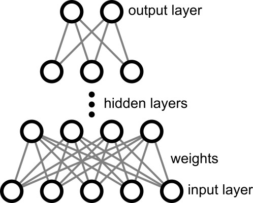
• layers of nodes (neurons) that apply a nonlinear activation functions $f,g,\ldots$ to a linear sum over inputs linked with weights $w_{ij}$ and constant biases $b_i$
  • $y_i = f\left(\sum_j w_{ij}~g\left(\sum_k w_{jk}x_k+b_j\right)+b_i\right)$
• originally inspired by brain, diverged, and more recently converged
• exponential expressive power of network depth vs breadth
• feature vector
  • input representation of data
• activation functions
  • sigmoid
    • $f(x) = 1/(1+e^{-x})$
    • between 0 and 1, good for binary output
  • tanh
    • $f(x) = (e^x-e^{-x})/(e^x+e^{-x})$
    • between -1 and 1, good for internal layers
  • ReLU (Rectified Linear Unit)
    • $f(x) = \mathrm{max}(0,x)$
    • fixes vanishing gradients, easier to compute
  • leaky ReLU
    • $f(x) = x$ for $x \ge 0$ and $f(x) = \alpha x$ for $x<0$ and small $\alpha$
    • fixes disappearing gradients
• hidden layers
  • internal layers between the inputs and outputs
• output units
  • linear for continuous regression
  • sigmoidal for binary classification
  • softmax for multiclass classification
• loss function
  • training goal for supervised learning
  • types
    • mean square error
      • difference between points
    • cross-entropy
      • difference between probability distributions
• return
  • training goal for reinforcement learning
  • games won, investment gain, ...

import numpy as np
import matplotlib.pyplot as plt
x = np.linspace(-3,3,100)
plt.plot(x,1/(1+np.exp(-x)),label='sigmoid')
plt.plot(x,np.tanh(x),label='tanh')
plt.plot(x,np.where(x < 0,0,x),label='ReLU')
plt.plot(x,np.where(x < 0,0.1*x,x),'--',label='leaky ReLU')
plt.legend()
plt.show()

Training

• back propagation
  • essential algorithm to propagate errors back through the network to perform the weight updates
• gradient descent
  • adjust weights to reduce loss function
• learning rate
  • the rate at which gradients are used to update weights
• stochastic gradient descent
  • for large data sets, adjust weights on random subsets of data points
  • batch = subset size
  • epoch = pass through entire data set
• momentum
  • add inertia to climb out of local minima
• ADAM (Adaptive Moment Estimation)
  • adjust learning rate for parameters individually
• L-BFGS
  • alternative optimizer using curvature as well as slope, which can converge faster and need less tuning
• early stopping
  • stop before loss finishes decreasing, to prevent over-fitting
• dropout
  • remove random selections of nodes during training to prevent over-fitting
• regularization
  • add penalty to control over-fitting
  • L2 for weight norm, L1 for weight sparsity
• pruning
  • removing nodes and links with small weights
• quantization
  • reducing the bits used to represent numbers, to decrease memory and computing requirements
• vanishing, diverging gradients
  • problems in deep networks
• inference
  • using models to make predictions after training

Taxonomy

• DNN: Deep Neural Network, MLP: Multi-Layer Perceptron
  • a neural network with hidden internal layers
• CNN: Convolutional Neural Network
  • a neural network that trains spatial filters to find features
• RNN Recurrent Neural Network
  • outputs are fed back to inputs, to be able to learn dynamics
• GAN: Generative Adversarial Network
  • a generator network tries to fool a discriminator network, learning how to generate data
• VAE: Variational Autoencoder
  • autoencoders connect and encoder network and a decoder network through a lower-dimensional intermediate layer
  • they can be used to find compact representations of the data, and to syntheize data
• LSTM: Long Short-Term Memory
  • adds memory to handle long-range dependencies
• Transformer
  • adds attention to handle long-range dependencies
• LLM: Large Language Model
  • trained on a large body of text
• surrogate model
  • a model trained to emulate a more complex computation, such as a physical simulation
  • Physics Informed Neural Network (PINN)
• AutoML
  • automated search over model architecture and hyperparameters
• Agentic AI
  • AI systems that can act autonomously on behalf of their users
• SVM: Support Vector Machine
  • alternative to neural networks
  • can perform better in large dimensions, and can be easier to interpret
  • training time is worse for large data sets, $\sim O(N^2)$
• vibe coding: programming with prompts to a LLM
  • issues: errors, hallucination, copyright, ...
  • need for understanding
  • frequently needs debugging

Models

• Hugging Face, Kaggle
  • huge model collections
• Edge Impulse, LiteRT
  • models targeting edge (embedded) devices
• ChatGPT, Claude, Gemini, ...
  • large language models that can write machine learning models
• ONNX
  • Open Neural Network Exchange interchange format

Frameworks

• scikit-learn
  • easy-to-use high-level routines
    • classifier
    • regression
• Jax
  • lower-level control, more scalable performance
  • Flax
    • simplified API for neural networks
  • HLO
    • code export from Jax
• PyTorch
  • widely used in machine learning research
• TensorFlow
  • TensorFlow.js

Examples

XOR

• trivial but historically important example because it can't be done linearly, showing all the essential steps
• [00,01,10,11] $\rightarrow$ [0,1,1,0]

scikit-learn

from sklearn.neural_network import MLPClassifier
import numpy as np
X = [[0,0],[0,1],[1,0],[1,1]]
y = [0,1,1,0]
classifier = MLPClassifier(solver='lbfgs',hidden_layer_sizes=(4),activation='tanh',random_state=1)
classifier.fit(X,y)
print(f"score: {classifier.score(X,y)}")
print("Predictions:")
np.c_[X,classifier.predict(X)]

score: 1.0
Predictions:

array([[0, 0, 0],
       [0, 1, 1],
       [1, 0, 1],
       [1, 1, 0]])

Jax

import jax
import jax.numpy as jnp
from jax import random,grad,jit
#
# init random key
#
key = random.PRNGKey(0)
#
# XOR training data
#
X = jnp.array([[0,0],[0,1],[1,0],[1,1]],dtype=jnp.int8)
y = jnp.array([0,1,1,0],dtype=jnp.int8).reshape(4,1)
#
# forward pass
#
@jit
def forward(params,layer_0):
    Weight1,bias1,Weight2,bias2 = params
    layer_1 = jnp.tanh(layer_0@Weight1+bias1)
    layer_2 = jax.nn.sigmoid(layer_1@Weight2+bias2)
    return layer_2
#
# loss function
#
@jit
def loss(params):
    ypred = forward(params,X)
    return jnp.mean((ypred-y)**2)
#
# gradient update step
#
@jit
def update(params,rate=0.5):
    gradient = grad(loss)(params)
    return jax.tree.map(lambda params,gradient:params-rate*gradient,params,gradient)
#
# parameter initialization
#
def init_params(key):
    key1,key2 = random.split(key)
    Weight1 = 0.5*random.normal(key1,(2,4))
    bias1 = jnp.zeros(4)
    Weight2 = 0.5*random.normal(key2,(4,1))
    bias2 = jnp.zeros(1)
    return (Weight1,bias1,Weight2,bias2)
#
# initialize parameters
#
params = init_params(key)
#
# training steps
#
for step in range(201):
    params = update(params,rate=10)
    if step%100 == 0:
        print(f"step {step:4d} loss={loss(params):.4f}")
#
# evaluate fit
#
pred = forward(params,X)
jnp.set_printoptions(precision=2)
print("\nPredictions:")
print(jnp.c_[X,pred])

step    0 loss=0.3047
step  100 loss=0.0008
step  200 loss=0.0004

Predictions:
[[0.   0.   0.01]
 [0.   1.   0.98]
 [1.   0.   0.98]
 [1.   1.   0.02]]

MNIST

• historically important non-trivial example

scikit-learn

from sklearn.neural_network import MLPClassifier
import numpy as np
xtrain = np.load('datasets/MNIST/xtrain.npy')
ytrain = np.load('datasets/MNIST/ytrain.npy')
xtest = np.load('datasets/MNIST/xtest.npy')
ytest = np.load('datasets/MNIST/ytest.npy')
print(f"read {xtrain.shape[1]} byte data records, {xtrain.shape[0]} training examples, {xtest.shape[0]} testing examples\n")
classifier = MLPClassifier(solver='adam',hidden_layer_sizes=(100),activation='relu',random_state=1,verbose=True,tol=0.05)
classifier.fit(xtrain,ytrain)
print(f"\ntest score: {classifier.score(xtest,ytest)}\n")
predictions = classifier.predict(xtest)
fig,axs = plt.subplots(1,5)
for i in range(5):
    axs[i].imshow(jnp.reshape(xtest[i],(28,28)))
    axs[i].axis('off')
    axs[i].set_title(f"predict: {predictions[i]}")
plt.tight_layout()
plt.show()

read 784 byte data records, 60000 training examples, 10000 testing examples

Iteration 1, loss = 3.36992820
Iteration 2, loss = 1.13264743
Iteration 3, loss = 0.67881654
Iteration 4, loss = 0.44722898
Iteration 5, loss = 0.31655389
Iteration 6, loss = 0.23663579
Iteration 7, loss = 0.19165519
Iteration 8, loss = 0.15617156
Iteration 9, loss = 0.13629980
Iteration 10, loss = 0.11865439
Iteration 11, loss = 0.11459503
Iteration 12, loss = 0.10146799
Iteration 13, loss = 0.09842103
Iteration 14, loss = 0.09300270
Iteration 15, loss = 0.08931920
Iteration 16, loss = 0.08818319
Iteration 17, loss = 0.09585389
Training loss did not improve more than tol=0.050000 for 10 consecutive epochs. Stopping.

test score: 0.958

Jax

import jax
import jax.numpy as jnp
from jax import random,grad,jit
import matplotlib.pyplot as plt
#
# hyperparameters
#
data_size = 28*28
hidden_size = data_size//10
output_size = 10
batch_size = 5000
train_steps = 25
learning_rate = 0.5
#
# init random key
#
key = random.PRNGKey(0)
#
# load MNIST data
#
xtrain = jnp.load('datasets/MNIST/xtrain.npy')
ytrain = jnp.load('datasets/MNIST/ytrain.npy')
xtest = jnp.load('datasets/MNIST/xtest.npy')
ytest = jnp.load('datasets/MNIST/ytest.npy')
print(f"read {xtrain.shape[1]} byte data records, {xtrain.shape[0]} training examples, {xtest.shape[0]} testing examples\n")
#
# forward pass
#
@jit
def forward(params,layer_0):
    Weight1,bias1,Weight2,bias2 = params
    layer_1 = jnp.tanh(layer_0@Weight1+bias1)
    layer_2 = layer_1@Weight2+bias2
    return layer_2
#
# loss function
#
@jit
def loss(params,xtrain,ytrain):
    logits = forward(params,xtrain)
    probs = jnp.exp(logits)/jnp.sum(jnp.exp(logits),axis=1,keepdims=True)
    error = 1-jnp.mean(probs[jnp.arange(len(ytrain)),ytrain])
    return error
#
# gradient update step
#
@jit
def update(params,xtrain,ytrain,rate):
    gradient = grad(loss)(params,xtrain,ytrain)
    return jax.tree.map(lambda params,gradient:params-rate*gradient,params,gradient)
#
# parameter initialization
#
def init_params(key,xsize,hidden,output):
    key1,key = random.split(key)
    Weight1 = 0.01*random.normal(key1,(xsize,hidden))
    bias1 = jnp.zeros(hidden)
    key2,key = random.split(key)
    Weight2 = 0.01*random.normal(key2,(hidden,output))
    bias2 = jnp.zeros(output)
    return (Weight1,bias1,Weight2,bias2)
#
# initialize parameters
#
params = init_params(key,data_size,hidden_size,output_size)
#
# train
#
print(f"starting loss: {loss(params,xtrain,ytrain):.3f}\n")
for batch in range(0,len(ytrain),batch_size):
    xbatch = xtrain[batch:batch+batch_size]
    ybatch = ytrain[batch:batch+batch_size]
    print(f"batch {batch}: ",end='')
    for step in range(train_steps):
        params = update(params,xbatch,ybatch,rate=learning_rate)
    print(f"loss {loss(params,xbatch,ybatch):.3f}")
#
# test
#
logits = forward(params,xtest)
probs = jnp.exp(logits)/jnp.sum(jnp.exp(logits),axis=1,keepdims=True)
error = 1-jnp.mean(probs[jnp.arange(len(ytest)),ytest])
print(f"\ntest loss: {error:.3f}\n")
#
# plot
#
fig,axs = plt.subplots(1,5)
for i in range(5):
    axs[i].imshow(jnp.reshape(xtest[i],(28,28)))
    axs[i].axis('off')
    axs[i].set_title(f"predict: {jnp.argmax(probs[i])}")
plt.tight_layout()
plt.show()

read 784 byte data records, 60000 training examples, 10000 testing examples

starting loss: 0.899

batch 0: loss 0.383
batch 5000: loss 0.239
batch 10000: loss 0.220
batch 15000: loss 0.163
batch 20000: loss 0.167
batch 25000: loss 0.104
batch 30000: loss 0.105
batch 35000: loss 0.092
batch 40000: loss 0.088
batch 45000: loss 0.089
batch 50000: loss 0.079
batch 55000: loss 0.053

test loss: 0.087

Assignment

• Fit a machine learning model to your data

Review

(c) Neil Gershenfeld for Fab Futures, 12/14/25