Luis Diaz-Faes - Fab Futures - Data Science

Home About A Industriosa

< Home

Day 2: Tools

Assignment 20/11/2025

Visualize your data set(s)

Read dataset

After reading this week’s documentation, watching the class video several times, and preparing a first set of sample datasets for the exercise, I started testing the code to open the CSV files and begin extracting data.

My datasets are separated by semicolons (;), so I need to keep that in mind when loading the CSVs. (More info in pandas.read_csv)

First dataset, daily data from 1/10/2008

import pandas as pd
from IPython.display import display, HTML


df = pd.read_csv('datasets/1363X-20081001-20251107.csv', delimiter=';')

display(HTML(f"<h4>Show first 10 columns</h4>"))
print(df.head(10)) ## the number limit the result to show

display(HTML(f"<h4>Table and column information:</h4>"))
df.info()

display(HTML(f"<h4>Show select data</h4>"))
df[["FECHA", "PRECIPITACION"]]

Show first 10 columns

      FECHA INDICATIVO     NOMBRE  ALTITUD  TMEDIA  PRECIPITACION  TMIN  \
0   1/10/08      1363X  AS PONTES      343    13.1            0.4   9.9   
1   2/10/08      1363X  AS PONTES      343    11.8            4.4   7.8   
2   3/10/08      1363X  AS PONTES      343     9.6            0.0   4.0   
3   4/10/08      1363X  AS PONTES      343     9.8            0.0   1.7   
4   5/10/08      1363X  AS PONTES      343    12.4            2.0   6.5   
5   6/10/08      1363X  AS PONTES      343    17.3            NaN  14.8   
6   7/10/08      1363X  AS PONTES      343    13.0            NaN   8.7   
7   8/10/08      1363X  AS PONTES      343    11.5            NaN   6.3   
8   9/10/08      1363X  AS PONTES      343    10.8            NaN   3.3   
9  10/10/08      1363X  AS PONTES      343    14.5            NaN   3.9   

  HORATMIN  TMAX HORATMAX  
0     7:00  16.3    14:52  
1    23:59  15.9    14:01  
2    23:59  15.2    11:39  
3   Varias  17.8    15:30  
4   Varias  18.3    13:39  
5   Varias  19.8    16:03  
6    23:00  17.3    13:00  
7    23:59  16.7    16:00  
8     6:00  18.2    13:00  
9     7:00  25.1    16:00  

Table and column information:

<class 'pandas.core.frame.DataFrame'>
RangeIndex: 6185 entries, 0 to 6184
Data columns (total 10 columns):
 #   Column         Non-Null Count  Dtype  
---  ------         --------------  -----  
 0   FECHA          6185 non-null   object 
 1   INDICATIVO     6185 non-null   object 
 2   NOMBRE         6185 non-null   object 
 3   ALTITUD        6185 non-null   int64  
 4   TMEDIA         6125 non-null   float64
 5   PRECIPITACION  5637 non-null   float64
 6   TMIN           6125 non-null   float64
 7   HORATMIN       6126 non-null   object 
 8   TMAX           6126 non-null   float64
 9   HORATMAX       6126 non-null   object 
dtypes: float64(4), int64(1), object(5)
memory usage: 483.3+ KB

Show select data

	FECHA	PRECIPITACION
0	1/10/08	0.4
1	2/10/08	4.4
2	3/10/08	0.0
3	4/10/08	0.0
4	5/10/08	2.0
...	...	...
6180	3/11/25	3.0
6181	4/11/25	1.2
6182	5/11/25	44.4
6183	6/11/25	27.4
6184	7/11/25	10.0

6185 rows × 2 columns

Second dataset, daily data from 07/05/2013

import pandas as pd
from IPython.display import display, HTML


df = pd.read_csv('datasets/1363X-20130507-20251031.csv', delimiter=';')

display(HTML(f"<h4>Show first 10 columns</h4>"))
print(df.head(10)) ## the number limit the result to show

display(HTML(f"<h4>Table and column information:</h4>"))
df.info()

display(HTML(f"<h4>Show select data</h4>"))
df[["Fecha", "Tmax", "Tmin", "TPrec"]]

Show first 10 columns

      Id       Fecha  Tmax  HTmax  Tmin  HTmin  Tmed  TPrec  Prec1  Prec2  \
0  1363X  2013-05-07  17.8  15:10  12.9  01:10  15.3   16.8   10.8    3.0   
1  1363X  2013-05-07  17.8  15:10  12.9  01:10  15.3   16.8   10.8    3.0   
2  1363X  2013-05-08  14.2  13:00  10.2  23:59  12.2    1.2    0.0    0.0   
3  1363X  2013-05-08  14.2  13:00  10.2  23:59  12.2    1.2    0.0    0.0   
4  1363X  2013-05-09  13.7  19:00   5.9  23:59   9.8    0.0    0.0    0.0   
5  1363X  2013-05-09  13.7  19:00   5.9  23:59   9.8    0.0    0.0    0.0   
6  1363X  2013-05-10  16.5  16:30   1.0  07:30   8.8    0.0    0.0    0.0   
7  1363X  2013-05-10  16.5  16:30   1.0  07:30   8.8    0.0    0.0    0.0   
8  1363X  2013-05-11  14.1  14:30   0.6  07:20   7.4    0.0    0.0    0.0   
9  1363X  2013-05-11  14.1  14:30   0.6  07:20   7.4    0.0    0.0    0.0   

   Prec3  Prec4  
0    3.0    0.0  
1    3.0    0.0  
2    1.2    0.0  
3    1.2    0.0  
4    0.0    0.0  
5    0.0    0.0  
6    0.0    0.0  
7    0.0    0.0  
8    0.0    0.0  
9    0.0    0.0  

Table and column information:

<class 'pandas.core.frame.DataFrame'>
RangeIndex: 8674 entries, 0 to 8673
Data columns (total 12 columns):
 #   Column  Non-Null Count  Dtype  
---  ------  --------------  -----  
 0   Id      8674 non-null   object 
 1   Fecha   8674 non-null   object 
 2   Tmax    8276 non-null   float64
 3   HTmax   8276 non-null   object 
 4   Tmin    8276 non-null   float64
 5   HTmin   8276 non-null   object 
 6   Tmed    8276 non-null   float64
 7   TPrec   7886 non-null   float64
 8   Prec1   8148 non-null   float64
 9   Prec2   8112 non-null   float64
 10  Prec3   8147 non-null   float64
 11  Prec4   8080 non-null   float64
dtypes: float64(8), object(4)
memory usage: 813.3+ KB

Show select data

	Fecha	Tmax	Tmin	TPrec
0	2013-05-07	17.8	12.9	16.8
1	2013-05-07	17.8	12.9	16.8
2	2013-05-08	14.2	10.2	1.2
3	2013-05-08	14.2	10.2	1.2
4	2013-05-09	13.7	5.9	0.0
...	...	...	...	...
8669	2025-10-27	19.8	0.8	0.0
8670	2025-10-28	14.7	5.0	8.0
8671	2025-10-29	14.7	5.0	8.0
8672	2025-10-30	16.0	7.7	0.8
8673	2025-10-31	17.8	13.4	27.0

8674 rows × 4 columns

import pandas as pd
from IPython.display import display, HTML


df = pd.read_csv('datasets/1363X-20190215-20200416.csv', delimiter=';')

display(HTML(f"<h4>Show first 10 columns</h4>"))
print(df.head(10)) ## the number limit the result to show

display(HTML(f"<h4>Table and column information:</h4>"))
df.info()

display(HTML(f"<h4>Show select data</h4>"))
df[["UTC", "Prec", "TempMin", "TempMax"]]

Show first 10 columns

      Id       Lon       Lat    Alt     Nombre                  UTC  Prec  \
0  1363X -7.861476  43.44597  343.0  AS PONTES  2019-02-15T21:00:00   0.0   
1  1363X -7.861476  43.44597  343.0  AS PONTES  2019-02-15T22:00:00   0.0   
2  1363X -7.861476  43.44597  343.0  AS PONTES  2019-02-15T23:00:00   0.0   
3  1363X -7.861476  43.44597  343.0  AS PONTES  2019-02-16T00:00:00   0.0   
4  1363X -7.861476  43.44597  343.0  AS PONTES  2019-02-16T01:00:00   0.0   
5  1363X -7.861476  43.44597  343.0  AS PONTES  2019-02-16T02:00:00   0.0   
6  1363X -7.861476  43.44597  343.0  AS PONTES  2019-02-16T03:00:00   0.0   
7  1363X -7.861476  43.44597  343.0  AS PONTES  2019-02-16T04:00:00   0.0   
8  1363X -7.861476  43.44597  343.0  AS PONTES  2019-02-16T05:00:00   0.0   
9  1363X -7.861476  43.44597  343.0  AS PONTES  2019-02-16T06:00:00   0.0   

    Hum  Temp  TempMin  TempMax  
0  81.0   7.3      7.3      8.9  
1  85.0   5.7      5.7      7.1  
2  89.0   4.3      4.3      5.4  
3  90.0   3.4      3.4      4.2  
4  93.0   2.6      2.6      3.2  
5  94.0   2.5      2.5      2.7  
6  94.0   1.7      1.7      2.3  
7  95.0   1.1      1.1      1.6  
8  96.0   0.7      0.7      1.1  
9  97.0   0.9      0.7      0.9  

Table and column information:

<class 'pandas.core.frame.DataFrame'>
RangeIndex: 52884 entries, 0 to 52883
Data columns (total 11 columns):
 #   Column   Non-Null Count  Dtype  
---  ------   --------------  -----  
 0   Id       52884 non-null  object 
 1   Lon      52884 non-null  float64
 2   Lat      52884 non-null  float64
 3   Alt      52884 non-null  float64
 4   Nombre   52884 non-null  object 
 5   UTC      52884 non-null  object 
 6   Prec     52556 non-null  float64
 7   Hum      52247 non-null  float64
 8   Temp     52248 non-null  float64
 9   TempMin  52248 non-null  float64
 10  TempMax  52248 non-null  float64
dtypes: float64(8), object(3)
memory usage: 4.4+ MB

Show select data

	UTC	Prec	TempMin	TempMax
0	2019-02-15T21:00:00	0.0	7.3	8.9
1	2019-02-15T22:00:00	0.0	5.7	7.1
2	2019-02-15T23:00:00	0.0	4.3	5.4
3	2019-02-16T00:00:00	0.0	3.4	4.2
4	2019-02-16T01:00:00	0.0	2.6	3.2
...	...	...	...	...
52879	2025-06-23T01:00:00+0000	0.0	13.5	14.3
52880	2025-06-23T02:00:00+0000	0.0	12.4	13.2
52881	2025-06-23T03:00:00+0000	0.0	11.8	12.2
52882	2025-06-23T04:00:00+0000	0.0	11.5	11.7
52883	2025-06-23T05:00:00+0000	0.0	11.4	11.5

52884 rows × 4 columns

Third dataset, hourly data from 15/02/2019

Visualize dataset

I use matplotlib.pyplot, a state-based interface to matplotlib. It provides an implicit, MATLAB-like, way of plotting. It also opens figures on your screen, and acts as the figure GUI manager.

Data from 2008 to 2025

This is my first test of visualize the data with values of csv file with data from 2008 to 2025.

import pandas as pd
import matplotlib.pyplot as plt

df = pd.read_csv("datasets/1363X-20081001-20251107.csv", sep=';')

df['FECHA'] = pd.to_datetime(df['FECHA'], format="%d/%m/%y", errors='coerce')
df = df.sort_values('FECHA')

plt.figure(figsize=(10,5))
plt.plot(df['FECHA'], df['PRECIPITACION'], label='PRECIPITACION')
plt.plot(df['FECHA'], df['TMEDIA'], label='TMEDIA')
plt.xlabel('Fecha')
plt.ylabel('Valor')
plt.legend()
plt.title('Temperatura media y precipitación por día')
plt.xticks(rotation=45)
plt.tight_layout()
plt.show()

### Data from 2008 to 2025 with interactive controls

I made same graph with temp max and min and add interactive controls for show or hide data.

# Static backend (no zoom/pan)
%matplotlib inline

import pandas as pd
import matplotlib.pyplot as plt
from ipywidgets import Checkbox, interact

# -------------------------------------------------------------
# 1. LOAD CSV (semicolon separator)
# -------------------------------------------------------------
df = pd.read_csv("datasets/1363X-20081001-20251107.csv", sep=";")
df["FECHA"] = pd.to_datetime(df["FECHA"], format="%d/%m/%y", dayfirst=True)

# -------------------------------------------------------------
# 2. AEMET COLORS
# -------------------------------------------------------------
color_tmedia = "#d7191c"
color_tmin   = "#fdae61"
color_tmax   = "#a50026"
color_prec   = "#2c7bb6"

# -------------------------------------------------------------
# 3. PLOT FUNCTION (NO LOESS)
# -------------------------------------------------------------
def plot_weather(show_tmedia, show_tmin, show_tmax, show_prec):

    d = df  # no date filtering

    fig, ax1 = plt.subplots(figsize=(14, 6))
    ax1.set_facecolor("#f7f7f7")
    ax1.grid(True, linestyle="--", linewidth=0.5, alpha=0.6)

    # Second axis for precipitation
    ax2 = ax1.twinx()

    # ----- TEMPERATURE (AX1) -----
    if show_tmedia:
        ax1.plot(d["FECHA"], d["TMEDIA"],
                 label="TMEDIA (avg temp)",
                 color=color_tmedia, linewidth=1)

    if show_tmin:
        ax1.plot(d["FECHA"], d["TMIN"],
                 label="TMIN (min temp)",
                 color=color_tmin, linewidth=1)

    if show_tmax:
        ax1.plot(d["FECHA"], d["TMAX"],
                 label="TMAX (max temp)",
                 color=color_tmax, linewidth=1)

    # ----- PRECIPITATION (AX2) -----
    if show_prec:
        ax2.bar(d["FECHA"], d["PRECIPITACION"],
                label="Precipitation",
                color=color_prec, alpha=0.35)

    # Axis labels
    ax1.set_xlabel("Date")
    ax1.set_ylabel("Temperature (°C)")
    ax2.set_ylabel("Precipitation (mm)")

    plt.title("Meteorological Data – AEMET Style (Dual Axis)")

    # Merge legends
    lines1, labels1 = ax1.get_legend_handles_labels()
    lines2, labels2 = ax2.get_legend_handles_labels()

    ax1.legend(lines1 + lines2, labels1 + labels2,
               loc="upper left",
               frameon=True, facecolor="white", edgecolor="#cccccc")

    plt.tight_layout()
    plt.show()


# -------------------------------------------------------------
# 4. INTERACTIVE CONTROLS
# -------------------------------------------------------------
interact(
    plot_weather,
    show_tmedia=Checkbox(value=True, description="Avg temp (TMEDIA)"),
    show_tmin=Checkbox(value=False, description="Min temp (TMIN)"),
    show_tmax=Checkbox(value=False, description="Max temp (TMAX)"),
    show_prec=Checkbox(value=True, description="Precipitation")
)

interactive(children=(Checkbox(value=True, description='Avg temp (TMEDIA)'), Checkbox(value=False, description…

<function __main__.plot_weather(show_tmedia, show_tmin, show_tmax, show_prec)>

Data from 2009

In this graph I show the temp min and max with temp media.

import pandas as pd
import matplotlib.pyplot as plt

# Load CSV with correct separator
df = pd.read_csv("datasets/1363X-20081001-20251107.csv", sep=";")

# Fix date format
df["FECHA"] = pd.to_datetime(df["FECHA"], format="%d/%m/%y", dayfirst=True)

# Convert numeric columns (AEMET CSV comes as text)
for col in ["TMEDIA", "TMIN", "TMAX", "PRECIPITACION"]:
    df[col] = pd.to_numeric(df[col], errors="coerce")

# Filter year 2009
df_2009 = df[df["FECHA"].dt.year == 2009]

# Plot
plt.figure(figsize=(14,6))

# Shaded area between TMIN and TMAX
plt.fill_between(
    df_2009["FECHA"],
    df_2009["TMIN"],
    df_2009["TMAX"],
    alpha=0.3
)

# TMEDIA line
plt.plot(df_2009["FECHA"], df_2009["TMEDIA"], linewidth=2)

plt.xlabel("Date")
plt.ylabel("Temperature (°C)")
plt.title("Temperature Range with Mean — Year 2009 - As Pontes (A Coruña - Spain)")
plt.tight_layout()
plt.show()

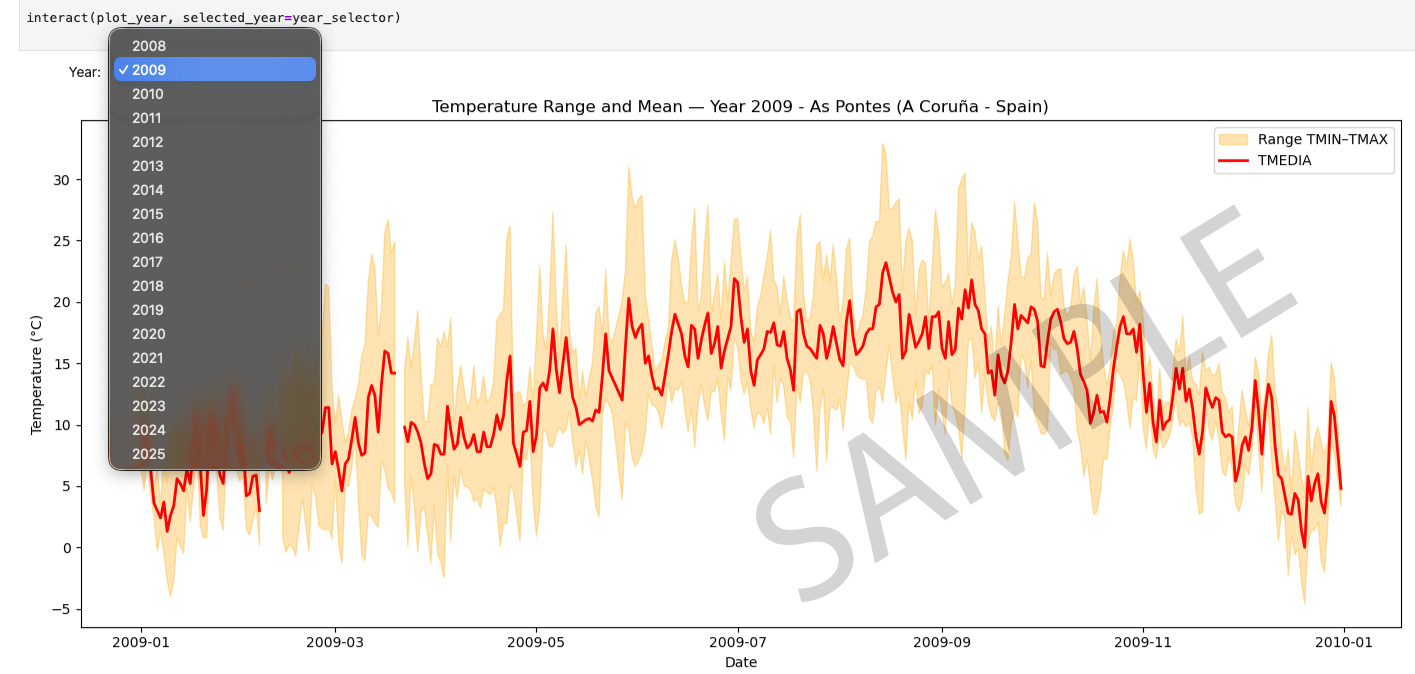
Data from any year

In this graph I also show the minimum and maximum temperature with the average temperature and I add a year selector, to see the data for each year.

import pandas as pd
import matplotlib.pyplot as plt
from ipywidgets import Dropdown, interact

# -------------------------------------------------------------
# 1. LOAD CSV WITH SEMICOLON SEPARATOR
# -------------------------------------------------------------
df = pd.read_csv("datasets/1363X-20081001-20251107.csv", sep=";")

# Date column
df["FECHA"] = pd.to_datetime(df["FECHA"], format="%d/%m/%y", dayfirst=True)

# Convert numeric columns
for col in ["TMEDIA", "TMIN", "TMAX", "PRECIPITACION"]:
    df[col] = pd.to_numeric(df[col], errors="coerce")

# Extract list of years
years = sorted(df["FECHA"].dt.year.unique())

# -------------------------------------------------------------
# 2. PLOT FUNCTION BY YEAR
# -------------------------------------------------------------
def plot_year(selected_year):

    d = df[df["FECHA"].dt.year == selected_year]

    plt.figure(figsize=(14,6))

    # Shaded area between TMIN and TMAX
    plt.fill_between(
        d["FECHA"],
        d["TMIN"],
        d["TMAX"],
        alpha=0.3,
        color="orange",
        label="Range TMIN–TMAX"
    )

    # TMEDIA line
    plt.plot(
        d["FECHA"],
        d["TMEDIA"],
        color="red",
        linewidth=2,
        label="TMEDIA"
    )

    plt.xlabel("Date")
    plt.ylabel("Temperature (°C)")
    plt.title(f"Temperature Range and Mean — Year {selected_year} - As Pontes (A Coruña - Spain)")
    plt.legend()
    plt.tight_layout()
    plt.show()

# -------------------------------------------------------------
# 3. DROPDOWN WIDGET FOR YEAR SELECTION
# -------------------------------------------------------------
year_selector = Dropdown(
    options=years,
    value=2009,
    description="Year:"
)

interact(plot_year, selected_year=year_selector)

interactive(children=(Dropdown(description='Year:', index=1, options=(np.int32(2008), np.int32(2009), np.int32…

<function __main__.plot_year(selected_year)>

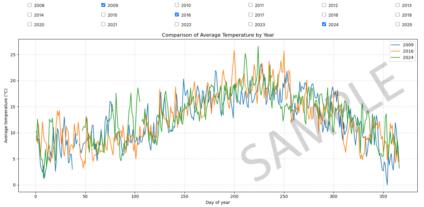
Year comparison tool

Here I compare data, allowing the user to select the years they want to compare.

import pandas as pd
import matplotlib.pyplot as plt
from ipywidgets import VBox, HBox, Checkbox, interactive_output

# -------------------------------------------------------------
# 1. LOAD CSV
# -------------------------------------------------------------
df = pd.read_csv("datasets/1363X-20081001-20251107.csv", sep=";")
df["FECHA"] = pd.to_datetime(df["FECHA"], format="%d/%m/%y", dayfirst=True)
df["TMEDIA"] = pd.to_numeric(df["TMEDIA"], errors="coerce")

# Extract year and day of year
df["YEAR"] = df["FECHA"].dt.year
df["DAY"] = df["FECHA"].dt.dayofyear

# List of years
years = sorted(df["YEAR"].unique())

# -------------------------------------------------------------
# 2. CREATE CHECKBOXES (keys MUST be strings)
# -------------------------------------------------------------
checkboxes = {str(year): Checkbox(value=False, description=str(year)) for year in years}

# Active 2009 and 2024 the first and last complete years with data.

checkboxes["2009"].value = True  # example: preselect 2009
checkboxes["2024"].value = True  # example: preselect 2024

# Layout (rows of 6 checkboxes)
ui = VBox([HBox(list(checkboxes.values())[i:i+6]) for i in range(0, len(checkboxes), 6)])


# -------------------------------------------------------------
# 3. PLOT FUNCTION (argument names must be strings)
# -------------------------------------------------------------
def plot_selected_years(**kwargs):

    plt.figure(figsize=(14,6))

    for year_str, active in kwargs.items():
        if active:
            year = int(year_str)
            d = df[df["YEAR"] == year]
            plt.plot(d["DAY"], d["TMEDIA"], linewidth=1.5, label=year_str)

    plt.xlabel("Day of year")
    plt.ylabel("Average temperature (°C)")
    plt.title("Comparison of Average Temperature by Year")
    plt.grid(True, linestyle="--", alpha=0.5)
    plt.legend()
    plt.tight_layout()
    plt.show()


# -------------------------------------------------------------
# 4. INTERACTIVE CONNECTION
# -------------------------------------------------------------
out = interactive_output(plot_selected_years, checkboxes)

display(ui, out)

VBox(children=(HBox(children=(Checkbox(value=False, description='2008'), Checkbox(value=True, description='200…

Output()

Comparing 2009 and 2024

These are the two years for which we have complete data. In this graph, we compare the values for each year.

import pandas as pd
import matplotlib.pyplot as plt

# -------------------------------------------------------------
# 1. LOAD CSV
# -------------------------------------------------------------
df = pd.read_csv("datasets/1363X-20081001-20251107.csv", sep=";")
df["FECHA"] = pd.to_datetime(df["FECHA"], format="%d/%m/%y", dayfirst=True)

# Convert numerical columns
for col in ["TMIN", "TMAX"]:
    df[col] = pd.to_numeric(df[col], errors="coerce")

# Add YEAR and DAY columns
df["YEAR"] = df["FECHA"].dt.year
df["DAY"] = df["FECHA"].dt.dayofyear

# -------------------------------------------------------------
# 2. FILTER YEARS 2009 AND 2024
# -------------------------------------------------------------
df_2009 = df[df["YEAR"] == 2009]
df_2024 = df[df["YEAR"] == 2024]

# -------------------------------------------------------------
# 3. PLOT COMPARISON
# -------------------------------------------------------------
plt.figure(figsize=(16,7))

# ---- TMAX ----
plt.plot(df_2009["DAY"], df_2009["TMAX"], color="red", label="TMAX 2009", linewidth=1.5)
plt.plot(df_2024["DAY"], df_2024["TMAX"], color="darkred", label="TMAX 2024", linewidth=1.5)

# ---- TMIN ----
plt.plot(df_2009["DAY"], df_2009["TMIN"], color="blue", label="TMIN 2009", linewidth=1.5)
plt.plot(df_2024["DAY"], df_2024["TMIN"], color="navy", label="TMIN 2024", linewidth=1.5)

# Formatting
plt.xlabel("Day of year")
plt.ylabel("Temperature (°C)")
plt.title("Comparison of Daily Minimum and Maximum Temperatures\n2009 vs 2024")
plt.grid(True, linestyle="--", alpha=0.5)
plt.legend()
plt.tight_layout()
plt.show()

Scatter plot for 2009 and 2024

These are the two years for which we have complete data. In this graph, we compare the values for each year, showing the maximum and minimum values.

import pandas as pd
import matplotlib.pyplot as plt

# -------------------------------------------------------------
# 1. LOAD CSV
# -------------------------------------------------------------
df = pd.read_csv("datasets/1363X-20081001-20251107.csv", sep=";")
df["FECHA"] = pd.to_datetime(df["FECHA"], format="%d/%m/%y", dayfirst=True)

# Convert numerical columns
for col in ["TMIN", "TMAX"]:
    df[col] = pd.to_numeric(df[col], errors="coerce")

# Create YEAR and DAY
df["YEAR"] = df["FECHA"].dt.year
df["DAY"] = df["FECHA"].dt.dayofyear

# Filter years
df_2009 = df[df["YEAR"] == 2009].set_index("DAY")
df_2024 = df[df["YEAR"] == 2024].set_index("DAY")

# Align by day of year
aligned = pd.DataFrame({
    "TMAX_2009": df_2009["TMAX"],
    "TMAX_2024": df_2024["TMAX"],
    "TMIN_2009": df_2009["TMIN"],
    "TMIN_2024": df_2024["TMIN"],
})

# Differences
aligned["DIFF_TMAX"] = aligned["TMAX_2024"] - aligned["TMAX_2009"]
aligned["DIFF_TMIN"] = aligned["TMIN_2024"] - aligned["TMIN_2009"]

# -------------------------------------------------------------
# 2. PLOT DIFFERENCES WITH COLOR CODING
# -------------------------------------------------------------
plt.figure(figsize=(16,8))

# --- TMAX Differences ---
for i, v in aligned["DIFF_TMAX"].dropna().items():
    color = "red" if v > 0 else "blue"
    plt.scatter(i, v, color=color, s=12)

# --- TMIN Differences ---
for i, v in aligned["DIFF_TMIN"].dropna().items():
    color = "green" if v > 0 else "purple"
    plt.scatter(i, v, color=color, s=12)

plt.axhline(0, color="black", linewidth=1)

plt.xlabel("Day of year")
plt.ylabel("Difference (°C)")
plt.title("Temperature Differences Between 2024 and 2009\nColored by Which Year Is Warmer/Colder")

plt.grid(True, linestyle="--", alpha=0.5)
plt.tight_layout()
plt.show()

import pandas as pd
import matplotlib.pyplot as plt

# -------------------------------------------------------------
# LOAD CSV
# -------------------------------------------------------------
df = pd.read_csv("datasets/1363X-20081001-20251107.csv", sep=";")
df["FECHA"] = pd.to_datetime(df["FECHA"], format="%d/%m/%y", dayfirst=True)

# Convert numbers
for col in ["TMIN", "TMAX"]:
    df[col] = pd.to_numeric(df[col], errors="coerce")

df["YEAR"] = df["FECHA"].dt.year
df["DAY"] = df["FECHA"].dt.dayofyear

# -------------------------------------------------------------
# FILTER 2009 AND 2024
# -------------------------------------------------------------
df_2009 = df[df["YEAR"] == 2009].set_index("DAY")
df_2024 = df[df["YEAR"] == 2024].set_index("DAY")

# Align by DAY
days = sorted(set(df_2009.index) & set(df_2024.index))

# Temperature differences
diff_tmax = df_2024.loc[days, "TMAX"] - df_2009.loc[days, "TMAX"]
diff_tmin = df_2024.loc[days, "TMIN"] - df_2009.loc[days, "TMIN"]

# Colors depending on higher or lower
colors_tmax = ["red" if x > 0 else "blue" for x in diff_tmax]
colors_tmin = ["red" if x > 0 else "blue" for x in diff_tmin]

# -------------------------------------------------------------
# PLOT
# -------------------------------------------------------------
plt.figure(figsize=(16,7))

# --- TMAX difference ---
plt.scatter(days, diff_tmax, c=colors_tmax, s=20, label="TMAX difference (2024 − 2009)")
plt.plot(days, diff_tmax, color="gray", alpha=0.4)

# --- TMIN difference ---
plt.scatter(days, diff_tmin, c=colors_tmin, s=20, marker="s", label="TMIN difference (2024 − 2009)")
plt.plot(days, diff_tmin, color="gray", alpha=0.4, linestyle="--")

# Labels and formatting
plt.axhline(0, color="black", linewidth=1)
plt.xlabel("Day of year", fontsize=12)
plt.ylabel("Temperature difference (°C)", fontsize=12)
plt.title("Temperature Difference Between 2024 and 2009\nPositive = 2024 warmer, Negative = 2024 colder", fontsize=15)
plt.grid(True, linestyle="--", alpha=0.5)
plt.legend()
plt.tight_layout()
plt.show()

Average temperature comparison between 2009 and 2024.

Graph showing how the average temperature in 2024 will vary compared to 2009.

import pandas as pd
import matplotlib.pyplot as plt

# -------------------------------------------------------------
# 1. Load CSV
# -------------------------------------------------------------
df = pd.read_csv("datasets/1363X-20081001-20251107.csv", sep=";")

# Convert date column
df["FECHA"] = pd.to_datetime(df["FECHA"], format="%d/%m/%y", dayfirst=True)

# Convert numeric columns
for col in ["TMEDIA", "TMIN", "TMAX", "PRECIPITACION"]:
    df[col] = pd.to_numeric(df[col], errors="coerce")

# Add year and day of year
df["YEAR"] = df["FECHA"].dt.year
df["DAY"] = df["FECHA"].dt.dayofyear

# -------------------------------------------------------------
# 2. Filter years 2009 and 2024
# -------------------------------------------------------------
df_2009 = df[df["YEAR"] == 2009].set_index("DAY")
df_2024 = df[df["YEAR"] == 2024].set_index("DAY")

# -------------------------------------------------------------
# 3. Align both years by day number
# -------------------------------------------------------------
aligned = pd.DataFrame({
    "TMEDIA_2009": df_2009["TMEDIA"],
    "TMEDIA_2024": df_2024["TMEDIA"]
})

# Calculate daily difference
aligned["DIFF"] = aligned["TMEDIA_2024"] - aligned["TMEDIA_2009"]

# -------------------------------------------------------------
# 4. Count how many days 2024 was warmer than 2009
# -------------------------------------------------------------
num_days_warmer = (aligned["DIFF"] > 0).sum()
print(f"Days where 2024 was warmer than 2009: {num_days_warmer}")

# -------------------------------------------------------------
# 5. Plot bar chart of differences
# -------------------------------------------------------------
plt.figure(figsize=(14,6))
plt.bar(aligned.index, aligned["DIFF"], color="orange")
plt.axhline(0, color="black", linewidth=1)

plt.xlabel("Day of year")
plt.ylabel("Temperature difference (°C)")
plt.title("TMEDIA Difference: 2024 - 2009")

plt.grid(True, linestyle="--", alpha=0.4)
plt.tight_layout()
plt.show()

Days where 2024 was warmer than 2009: 178

Histogram of temperature differences 2009 - 2024.

import pandas as pd
import matplotlib.pyplot as plt

# -------------------------------------------------------------
# 1. Load the CSV
# -------------------------------------------------------------
df = pd.read_csv("datasets/1363X-20081001-20251107.csv", sep=";")

# Parse date column
df["FECHA"] = pd.to_datetime(df["FECHA"], format="%d/%m/%y", dayfirst=True)

# Convert numeric columns
df["TMEDIA"] = pd.to_numeric(df["TMEDIA"], errors="coerce")

# Add YEAR and DAY
df["YEAR"] = df["FECHA"].dt.year
df["DAY"] = df["FECHA"].dt.dayofyear

# -------------------------------------------------------------
# 2. Filter years 2009 and 2024
# -------------------------------------------------------------
df_2009 = df[df["YEAR"] == 2009].set_index("DAY")
df_2024 = df[df["YEAR"] == 2024].set_index("DAY")

# -------------------------------------------------------------
# 3. Align the two years day-by-day
# -------------------------------------------------------------
aligned = pd.DataFrame({
    "TMEDIA_2009": df_2009["TMEDIA"],
    "TMEDIA_2024": df_2024["TMEDIA"]
})

# Difference (2024 - 2009)
aligned["DIFF"] = aligned["TMEDIA_2024"] - aligned["TMEDIA_2009"]

# -------------------------------------------------------------
# 4. Mean temperature change
# -------------------------------------------------------------
mean_change = aligned["DIFF"].mean()
print(f"Mean temperature change (2024 - 2009): {mean_change:.2f} °C")

# -------------------------------------------------------------
# 5. Plot histogram of differences
# -------------------------------------------------------------
plt.figure(figsize=(10,5))
plt.hist(aligned["DIFF"].dropna(), bins=30, color="orange", edgecolor="black")

# Vertical line at the mean difference
plt.axvline(mean_change, color="red", linestyle="--", linewidth=2,
            label=f"Mean change = {mean_change:.2f} °C")

plt.xlabel("Temperature Difference (°C)")
plt.ylabel("Frequency")
plt.title("Histogram of Temperature Differences (TMEDIA 2024 - 2009)")
plt.legend()
plt.grid(True, linestyle="--", alpha=0.4)
plt.tight_layout()
plt.show()

Mean temperature change (2024 - 2009): 0.62 °C

Average Temperature difference

The graph shows the difference in average temperature (TMEDIA) for each year compared with the year 2024.

import pandas as pd
import matplotlib.pyplot as plt

# -------------------------------------------------------------
# 1. Load CSV
# -------------------------------------------------------------
df = pd.read_csv("datasets/1363X-20081001-20251107.csv", sep=";")

# Convert dates and numeric columns
df["FECHA"] = pd.to_datetime(df["FECHA"], format="%d/%m/%y", dayfirst=True)
df["TMEDIA"] = pd.to_numeric(df["TMEDIA"], errors="coerce")
df["YEAR"] = df["FECHA"].dt.year
df["DAY"] = df["FECHA"].dt.dayofyear

# -------------------------------------------------------------
# 2. Filter 2024
# -------------------------------------------------------------
df_2024 = df[df["YEAR"] == 2024].set_index("DAY")["TMEDIA"]

# -------------------------------------------------------------
# 3. Compare every year 2009–2023 against 2024
# -------------------------------------------------------------
results = {}

for year in range(2009, 2024):
    df_y = df[df["YEAR"] == year].set_index("DAY")["TMEDIA"]
    
    # Align the days
    aligned = pd.DataFrame({
        "YEAR": df_y,
        "Y2024": df_2024
    }).dropna()
    
    # Compute mean difference (2024 - year)
    diff = (aligned["Y2024"] - aligned["YEAR"]).mean()
    results[year] = diff

# Convert to DataFrame
diff_df = pd.DataFrame.from_dict(results, orient="index", columns=["Difference_2024_minus_year"])
print(diff_df)

# -------------------------------------------------------------
# 4. Plot bar chart
# -------------------------------------------------------------
plt.figure(figsize=(12,6))
plt.bar(diff_df.index, diff_df["Difference_2024_minus_year"], color="orange", edgecolor="black")

plt.axhline(0, color="black", linewidth=1)
plt.xlabel("Year")
plt.ylabel("Temperature Difference (°C)")
plt.title("Average Temperature Difference vs 2024 (TMEDIA)")
plt.grid(True, linestyle="--", alpha=0.4)

plt.tight_layout()
plt.show()

      Difference_2024_minus_year
2009                    0.621212
2010                    0.899096
2011                   -0.058982
2012                    0.647774
2013                    0.747576
2014                    0.151840
2015                    0.004923
2016                    0.388131
2017                   -0.181845
2018                    0.088024
2019                    0.319520
2020                   -0.244345
2021                    0.442262
2022                   -0.603503
2023                   -1.080299