Luis Diaz-Faes - Fab Futures - Data Science

Home About A Industriosa

Day 8: Presentation

import pandas as pd
from IPython.display import display, HTML


df = pd.read_csv('datasets/1363X-20190215-20200416.csv', delimiter=';')

display(HTML(f"<h4>Show first 10 columns</h4>"))
print(df.head(10)) ## the number limit the result to show

display(HTML(f"<h4>Table and column information:</h4>"))
df.info()

display(HTML(f"<h4>Show select data</h4>"))
df[["UTC", "Temp", "Prec", "Hum"]]

Show first 10 columns

      Id       Lon       Lat    Alt     Nombre                  UTC  Prec  \
0  1363X -7.861476  43.44597  343.0  AS PONTES  2019-02-15T21:00:00   0.0   
1  1363X -7.861476  43.44597  343.0  AS PONTES  2019-02-15T22:00:00   0.0   
2  1363X -7.861476  43.44597  343.0  AS PONTES  2019-02-15T23:00:00   0.0   
3  1363X -7.861476  43.44597  343.0  AS PONTES  2019-02-16T00:00:00   0.0   
4  1363X -7.861476  43.44597  343.0  AS PONTES  2019-02-16T01:00:00   0.0   
5  1363X -7.861476  43.44597  343.0  AS PONTES  2019-02-16T02:00:00   0.0   
6  1363X -7.861476  43.44597  343.0  AS PONTES  2019-02-16T03:00:00   0.0   
7  1363X -7.861476  43.44597  343.0  AS PONTES  2019-02-16T04:00:00   0.0   
8  1363X -7.861476  43.44597  343.0  AS PONTES  2019-02-16T05:00:00   0.0   
9  1363X -7.861476  43.44597  343.0  AS PONTES  2019-02-16T06:00:00   0.0   

    Hum  Temp  TempMin  TempMax  
0  81.0   7.3      7.3      8.9  
1  85.0   5.7      5.7      7.1  
2  89.0   4.3      4.3      5.4  
3  90.0   3.4      3.4      4.2  
4  93.0   2.6      2.6      3.2  
5  94.0   2.5      2.5      2.7  
6  94.0   1.7      1.7      2.3  
7  95.0   1.1      1.1      1.6  
8  96.0   0.7      0.7      1.1  
9  97.0   0.9      0.7      0.9  

Table and column information:

<class 'pandas.core.frame.DataFrame'>
RangeIndex: 52884 entries, 0 to 52883
Data columns (total 11 columns):
 #   Column   Non-Null Count  Dtype  
---  ------   --------------  -----  
 0   Id       52884 non-null  object 
 1   Lon      52884 non-null  float64
 2   Lat      52884 non-null  float64
 3   Alt      52884 non-null  float64
 4   Nombre   52884 non-null  object 
 5   UTC      52884 non-null  object 
 6   Prec     52556 non-null  float64
 7   Hum      52247 non-null  float64
 8   Temp     52248 non-null  float64
 9   TempMin  52248 non-null  float64
 10  TempMax  52248 non-null  float64
dtypes: float64(8), object(3)
memory usage: 4.4+ MB

Show select data

	UTC	Temp	Prec	Hum
0	2019-02-15T21:00:00	7.3	0.0	81.0
1	2019-02-15T22:00:00	5.7	0.0	85.0
2	2019-02-15T23:00:00	4.3	0.0	89.0
3	2019-02-16T00:00:00	3.4	0.0	90.0
4	2019-02-16T01:00:00	2.6	0.0	93.0
...	...	...	...	...
52879	2025-06-23T01:00:00+0000	13.5	0.0	91.0
52880	2025-06-23T02:00:00+0000	12.4	0.0	92.0
52881	2025-06-23T03:00:00+0000	11.8	0.0	94.0
52882	2025-06-23T04:00:00+0000	11.5	0.0	95.0
52883	2025-06-23T05:00:00+0000	11.4	0.0	95.0

52884 rows × 4 columns

import pandas as pd
import numpy as np
import matplotlib.pyplot as plt

from matplotlib.gridspec import GridSpec
from sklearn.preprocessing import StandardScaler
from sklearn.cluster import KMeans
from sklearn.mixture import GaussianMixture
from sklearn.decomposition import PCA

# ----------------------------------------------------
# 1. LOAD AND PREPARE DATA
# ----------------------------------------------------
df = pd.read_csv("datasets/1363X-20190215-20200416.csv", sep=";")

df["UTC"] = pd.to_datetime(df["UTC"], errors="coerce", utc=True)
df = df.dropna(subset=["UTC", "Temp", "Hum", "Prec"]).copy()
df = df.sort_values("UTC").reset_index(drop=True)

df["YEAR"] = df["UTC"].dt.year
df["DATE"] = df["UTC"].dt.date
df["HOUR"] = df["UTC"].dt.hour

# Focus on 2019–2024
df = df[df["YEAR"].between(2019, 2024)].copy()

print("Years present:", sorted(df["YEAR"].unique()))
print("Total rows:", len(df))

# Fog-like condition
fog_mask = (
    (df["Hum"] >= 95.0) &
    (df["Temp"] >= -2.0) &
    (df["Temp"] <= 15.0)
)
df["FOG_FLAG"] = fog_mask
df["RAIN_FLAG"] = df["Prec"] > 0

# ----------------------------------------------------
# 2. YEARLY SUMMARY (for humidity and fog)
# ----------------------------------------------------
summary = (
    df.groupby("YEAR")
    .agg(
        temp_mean=("Temp", "mean"),
        hum_mean=("Hum", "mean"),
        hum_median=("Hum", "median"),
        hum_p95=("Hum", lambda x: np.percentile(x, 95)),
        fog_hours=("FOG_FLAG", "sum"),
        total_hours=("FOG_FLAG", "size"),
        rainy_hours=("RAIN_FLAG", "sum"),
        prec_mean=("Prec", "mean")
    )
    .reset_index()
)

summary["fog_pct"] = 100.0 * summary["fog_hours"] / summary["total_hours"]

years_arr = summary["YEAR"].values

# ----------------------------------------------------
# 3. FOG SUBSET AND TRANSFORMS (K-means, GMM, PCA)
# ----------------------------------------------------
df_fog = df[df["FOG_FLAG"]].copy()
print("Fog-like hourly records:", len(df_fog))

# Features for clustering / density: (Hum, Temp)
X_fog_raw = df_fog[["Hum", "Temp"]].values
scaler_fog = StandardScaler()
X_fog = scaler_fog.fit_transform(X_fog_raw)

# --- K-means on fog (Hum, Temp) ---
K_kmeans = 4
K_kmeans = min(K_kmeans, len(df_fog))  # safety
kmeans = KMeans(n_clusters=K_kmeans, random_state=0, n_init=10)
labels_km = kmeans.fit_predict(X_fog)

centers_scaled = kmeans.cluster_centers_
centers = scaler_fog.inverse_transform(centers_scaled)

# --- GMM density on fog (Hum, Temp) ---
max_components = min(5, len(df_fog))
bics = []
gmms = []
components_range = range(1, max_components + 1)

for m in components_range:
    gmm = GaussianMixture(
        n_components=m,
        covariance_type="full",
        random_state=0
    )
    gmm.fit(X_fog)
    gmms.append(gmm)
    bics.append(gmm.bic(X_fog))

best_idx = int(np.argmin(bics))
best_M = components_range[best_idx]
gmm_best = gmms[best_idx]
print("Best GMM components for fog (by BIC):", best_M)

# Grid for density
hum_min, hum_max = df_fog["Hum"].min(), df_fog["Hum"].max()
temp_min, temp_max = df_fog["Temp"].min(), df_fog["Temp"].max()

hum_vals = np.linspace(hum_min, hum_max, 80)
temp_vals = np.linspace(temp_min, temp_max, 80)
HH, TT = np.meshgrid(hum_vals, temp_vals)
grid_points = np.column_stack([HH.ravel(), TT.ravel()])
grid_scaled = scaler_fog.transform(grid_points)
logp = gmm_best.score_samples(grid_scaled)
P = np.exp(logp).reshape(HH.shape)

# --- PCA on fog (Hum, Temp, Prec) ---
X_pca_raw = df_fog[["Hum", "Temp", "Prec"]].values
scaler_pca = StandardScaler()
X_pca_scaled = scaler_pca.fit_transform(X_pca_raw)

pca = PCA(n_components=2)
X_pca = pca.fit_transform(X_pca_scaled)
expl_var = pca.explained_variance_ratio_

# ----------------------------------------------------
# 4. COMPRESSED-SENSING STYLE RECONSTRUCTION (TEMP)
# ----------------------------------------------------
df_2019 = df[df["YEAR"] == 2019].copy()
temp_series_2019 = df_2019["Temp"].values
N_max = 512
N = min(N_max, len(temp_series_2019))
signal = temp_series_2019[:N]
t_seg = np.arange(N)

# FFT and sparse reconstruction
F = np.fft.rfft(signal)
K_sparse = 20
idx_sorted = np.argsort(np.abs(F))[::-1]
F_sparse = np.zeros_like(F, dtype=complex)
F_sparse[idx_sorted[:K_sparse]] = F[idx_sorted[:K_sparse]]
signal_recon = np.fft.irfft(F_sparse, n=N)
error_signal = signal - signal_recon

# ----------------------------------------------------
# 5. BUILD 1920x1080 SUMMARY FIGURE
# ----------------------------------------------------
# 1920x1080 at 100 dpi -> 19.2 x 10.8 inches
fig = plt.figure(figsize=(19.2, 10.8), dpi=100)
gs = GridSpec(2, 3, figure=fig)

# --- Panel 1: yearly mean Temp & Hum ---
ax1 = fig.add_subplot(gs[0, 0])
ax1.plot(summary["YEAR"], summary["temp_mean"], marker="o", label="Mean Temp (°C)")
ax1.plot(summary["YEAR"], summary["hum_mean"], marker="s", label="Mean Hum (%)")
ax1.set_xlabel("Year")
ax1.set_ylabel("Value")
ax1.set_title("Yearly mean temperature and humidity\n(2019–2024)")
ax1.grid(True, alpha=0.3)
ax1.set_xticks(years_arr)
ax1.legend(fontsize=9)

# --- Panel 2: humidity + fog% with plant shutdown ---
ax2 = fig.add_subplot(gs[0, 1])
ax2.plot(summary["YEAR"], summary["hum_mean"], marker="o", linewidth=2, label="Mean Humidity")
ax2.fill_between(
    summary["YEAR"],
    summary["hum_median"],
    summary["hum_p95"],
    alpha=0.15,
    label="Median–95th percentile"
)
ax2.set_xlabel("Year")
ax2.set_ylabel("Humidity (%)")
ax2.set_title("Humidity and fog-like hours\nAs Pontes power plant shutdown (2023)")
ax2.grid(True, alpha=0.3)
ax2.set_xticks(years_arr)

ax2.axvline(x=2023, color="gray", linestyle="--", alpha=0.7)

ax2b = ax2.twinx()
ax2b.plot(summary["YEAR"], summary["fog_pct"], marker="s", linewidth=2, color="tab:red",
          label="Fog-like hours (%)")
ax2b.set_ylabel("Fog-like hours (%)", color="tab:red")
ax2b.tick_params(axis="y", labelcolor="tab:red")

lines1, labels1 = ax2.get_legend_handles_labels()
lines2, labels2 = ax2b.get_legend_handles_labels()
ax2.legend(lines1 + lines2, labels1 + labels2, loc="upper left", fontsize=8)

# --- Panel 3: K-means clustering of fog (Hum, Temp) ---
ax3 = fig.add_subplot(gs[0, 2])
sc3 = ax3.scatter(
    df_fog["Hum"],
    df_fog["Temp"],
    c=labels_km,
    s=5,
    alpha=0.5
)
ax3.scatter(
    centers[:, 0],
    centers[:, 1],
    marker="X",
    s=80,
    edgecolor="white",
    linewidth=1.0,
    c=range(K_kmeans)
)
ax3.set_xlabel("Humidity (Hum, %)")
ax3.set_ylabel("Temperature (Temp, °C)")
ax3.set_title("Fog regimes: K-means clustering\nin (Hum, Temp) space")
ax3.grid(True, alpha=0.3)

# --- Panel 4: GMM density for fog (Hum, Temp) ---
ax4 = fig.add_subplot(gs[1, 0])
cont = ax4.contourf(HH, TT, P, levels=15)
fig.colorbar(cont, ax=ax4, fraction=0.046, pad=0.04)
ax4.scatter(
    df_fog["Hum"],
    df_fog["Temp"],
    s=3,
    alpha=0.25,
    edgecolors="none"
)
ax4.set_xlabel("Humidity (Hum, %)")
ax4.set_ylabel("Temperature (Temp, °C)")
ax4.set_title(f"GMM density estimation for fog\nM = {best_M} components")
ax4.grid(True, alpha=0.3)

# --- Panel 5: PCA of fog (Hum, Temp, Prec) ---
ax5 = fig.add_subplot(gs[1, 1])
ax5.scatter(
    X_pca[:, 0],
    X_pca[:, 1],
    s=5,
    alpha=0.6
)
ax5.set_xlabel(f"PC1 ({expl_var[0]*100:.1f}% var)")
ax5.set_ylabel(f"PC2 ({expl_var[1]*100:.1f}% var)")
ax5.set_title("PCA of fog conditions\n(Hum, Temp, Prec)")
ax5.grid(True, alpha=0.3)

# --- Panel 6: compressed-sensing style reconstruction (Temp) ---
ax6 = fig.add_subplot(gs[1, 2])
ax6.plot(t_seg, signal, label="Original Temp (2019 segment)", linewidth=1.0)
ax6.plot(t_seg, signal_recon, label=f"Reconstructed (K={K_sparse} Fourier coeffs)",
         linewidth=1.0)
ax6.set_xlabel("Sample index")
ax6.set_ylabel("Temp (°C)")
ax6.set_title("Sparse Fourier reconstruction of temperature")
ax6.grid(True, alpha=0.3)
ax6.legend(fontsize=8)

# Overall title (optional)
fig.suptitle("Data Science for Fab Futures – As Pontes climate analysis (2019–2024)",
             fontsize=16, y=0.98)

plt.tight_layout(rect=[0, 0, 1, 0.96])
plt.show()

Years present: [np.int32(2019), np.int32(2020), np.int32(2021), np.int32(2022), np.int32(2023), np.int32(2024)]
Total rows: 43343
Fog-like hourly records: 11988
Best GMM components for fog (by BIC): 5

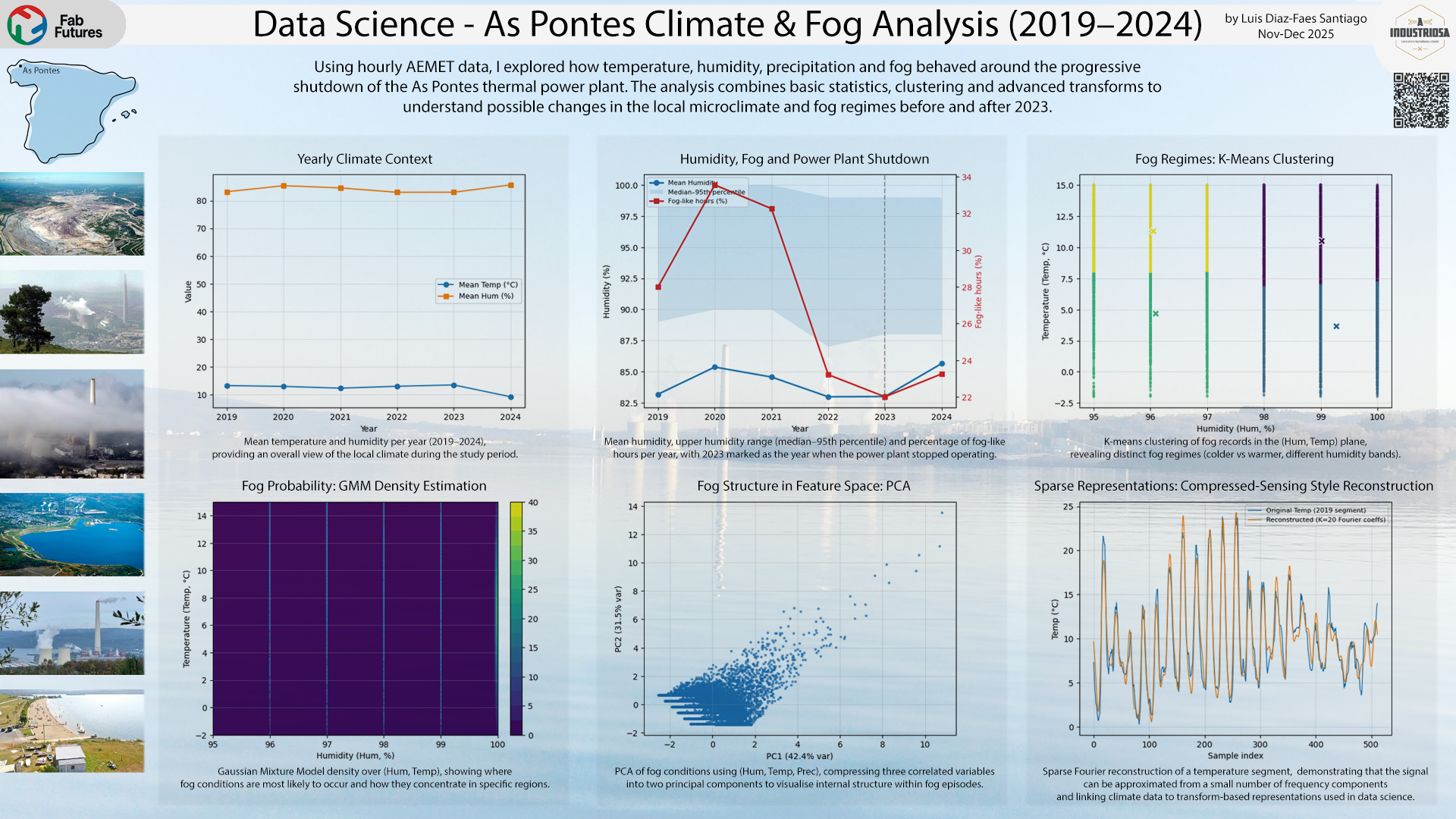
The summary figure brings together the main ideas explored during the course using my AEMET data for As Pontes (2019–2024):

• Top left: yearly mean temperature and humidity, showing the overall climate context of the period.
• Top centre: mean humidity and percentage of fog-like hours per year, with a vertical line marking 2023, when the As Pontes thermal power plant stopped operating and its cooling towers no longer contributed extra moisture to the atmosphere.
• Top right: a K-means clustering of fog records in the (Hum, Temp) plane, revealing distinct fog regimes (colder vs slightly warmer, different humidity bands).
• Bottom left: a GMM density estimation over the same (Hum, Temp) space, showing where fog conditions are most likely to occur.
• Bottom centre: a PCA projection of fog conditions using (Hum, Temp, Prec), compressing three correlated variables into two principal components and highlighting structure within fog episodes.
• Bottom right: a compressed-sensing style reconstruction of temperature, where a short segment of the 2019 series is rebuilt from only a small number of Fourier coefficients, illustrating sparsity and transform-based representations.

Together, these panels summarise the path of the project: from basic statistics and visualisation, through clustering and probabilistic modelling of fog, to advanced transforms (PCA, density estimation and sparse reconstructions) used to explore how local climate patterns may have changed around the shutdown of the As Pontes power plant.

See you in the Fab Labs of the Future.