Anith Ghalley - Fab Futures - Data Science

Home About

Week 3 : Probabilities

Assignment

• Investigate the probability distribution of your data
• Set up template notebooks and slides for your data set analysis

Template notebook and slides

The task was to prepare a notebook with the analysis of your data set (Currently need to make a dummpy notebook for future work), store it in your repo, and call it presentation.ipynb

1. Create a notebook inside the folder.

2. Make sure you select to start the kernel as well

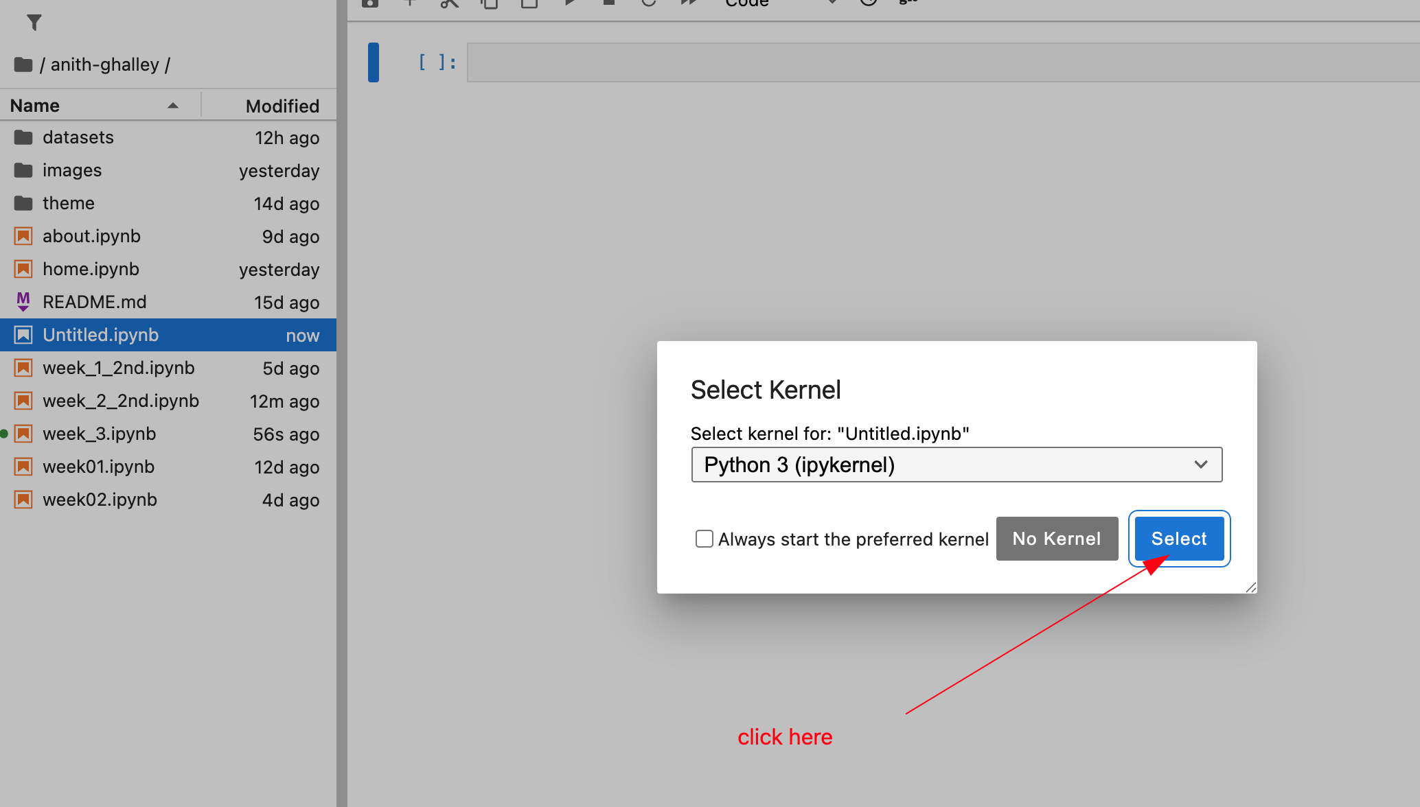
3. Rename the note book as presentation.ipynb

include a 1920x1080 summary slide describing you, your data, and your analysis, store it your repo's images folder, and call it presentation.png

Then to create a dummy presentation slide, i used Canva to make the custom size as shared below:

Next make sure to maintain this size 1920x1080 px

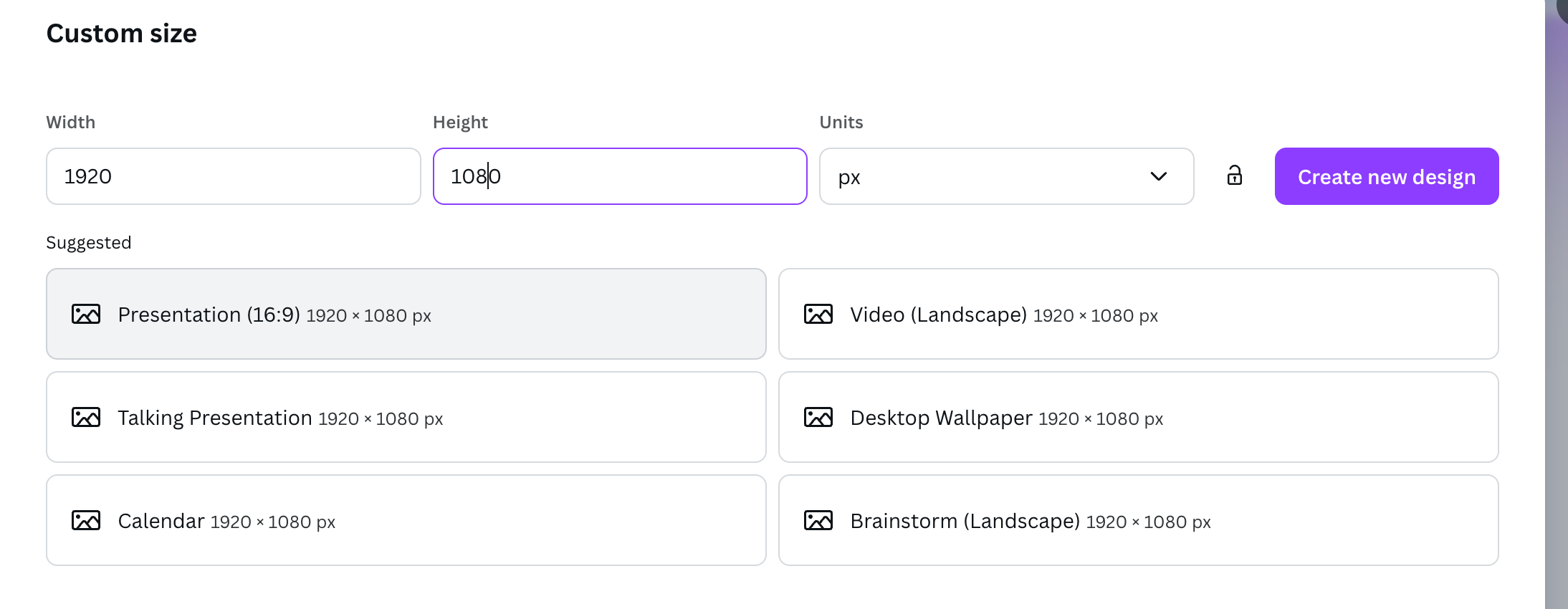
Then you can create a dummy slide and download it.

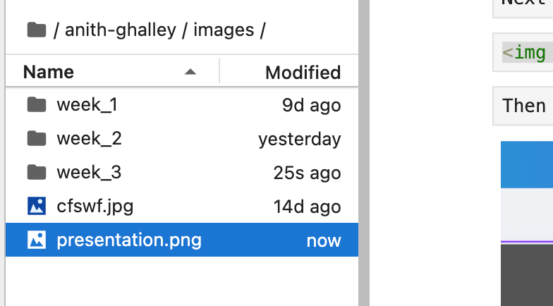
Save the presentation.png inside the image folder

The presentation is added to the presentation.ipynb file

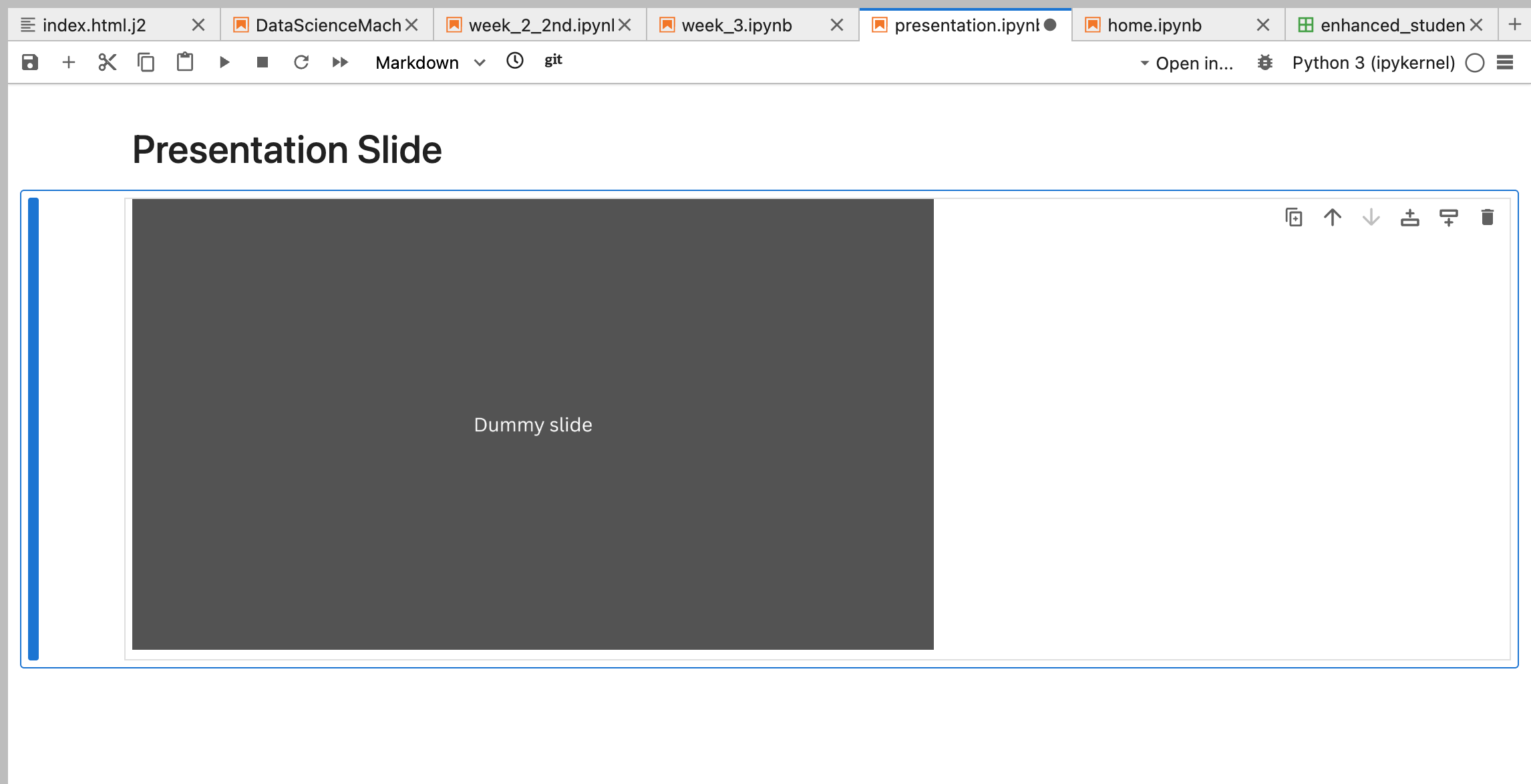
And the notebook is also linked to my home page.

Probability Distribution

To invistigate my datasets probability distribution i have documented my work here

In simple terms, "investigate" means to examine the data's shape and characteristics to determine what kind of mathematical model best describes it, and whether you can use simple statistics (like the mean and variance of a single distribution) or if you need advanced techniques (like mixture models).

import pandas as pd

df = pd.read_csv('datasets/enhanced_student_habits_performance_dataset.csv')  # load dataset
print(df.head())                        # preview data

   student_id  age  gender             major  study_hours_per_day  \
0      100000   26    Male  Computer Science             7.645367   
1      100001   28    Male              Arts             5.700000   
2      100002   17    Male              Arts             2.400000   
3      100003   27   Other        Psychology             3.400000   
4      100004   25  Female          Business             4.700000   

   social_media_hours  netflix_hours part_time_job  attendance_percentage  \
0                 3.0            0.1           Yes                   70.3   
1                 0.5            0.4            No                   88.4   
2                 4.2            0.7            No                   82.1   
3                 4.6            2.3           Yes                   79.3   
4                 0.8            2.7           Yes                   62.9   

   sleep_hours  ... screen_time  study_environment access_to_tutoring  \
0          6.2  ...        10.9  Co-Learning Group                Yes   
1          7.2  ...         8.3  Co-Learning Group                Yes   
2          9.2  ...         8.0            Library                Yes   
3          4.2  ...        11.7  Co-Learning Group                Yes   
4          6.5  ...         9.4         Quiet Room                Yes   

  family_income_range  parental_support_level motivation_level  \
0                High                       9                7   
1                 Low                       7                2   
2                High                       3                9   
3                 Low                       5                3   
4              Medium                       9                1   

   exam_anxiety_score  learning_style  time_management_score exam_score  
0                   8         Reading                    3.0        100  
1                  10         Reading                    6.0         99  
2                   6     Kinesthetic                    7.6         98  
3                  10         Reading                    3.2        100  
4                  10         Reading                    7.1         98  

[5 rows x 31 columns]

print(df.info())                        # check column types

<class 'pandas.core.frame.DataFrame'>
RangeIndex: 80000 entries, 0 to 79999
Data columns (total 31 columns):
 #   Column                         Non-Null Count  Dtype  
---  ------                         --------------  -----  
 0   student_id                     80000 non-null  int64  
 1   age                            80000 non-null  int64  
 2   gender                         80000 non-null  object 
 3   major                          80000 non-null  object 
 4   study_hours_per_day            80000 non-null  float64
 5   social_media_hours             80000 non-null  float64
 6   netflix_hours                  80000 non-null  float64
 7   part_time_job                  80000 non-null  object 
 8   attendance_percentage          80000 non-null  float64
 9   sleep_hours                    80000 non-null  float64
 10  diet_quality                   80000 non-null  object 
 11  exercise_frequency             80000 non-null  int64  
 12  parental_education_level       80000 non-null  object 
 13  internet_quality               80000 non-null  object 
 14  mental_health_rating           80000 non-null  float64
 15  extracurricular_participation  80000 non-null  object 
 16  previous_gpa                   80000 non-null  float64
 17  semester                       80000 non-null  int64  
 18  stress_level                   80000 non-null  float64
 19  dropout_risk                   80000 non-null  object 
 20  social_activity                80000 non-null  int64  
 21  screen_time                    80000 non-null  float64
 22  study_environment              80000 non-null  object 
 23  access_to_tutoring             80000 non-null  object 
 24  family_income_range            80000 non-null  object 
 25  parental_support_level         80000 non-null  int64  
 26  motivation_level               80000 non-null  int64  
 27  exam_anxiety_score             80000 non-null  int64  
 28  learning_style                 80000 non-null  object 
 29  time_management_score          80000 non-null  float64
 30  exam_score                     80000 non-null  int64  
dtypes: float64(10), int64(9), object(12)
memory usage: 18.9+ MB
None

print(df.describe())                    # summary stats

          student_id           age  study_hours_per_day  social_media_hours  \
count   80000.000000  80000.000000         80000.000000        80000.000000   
mean   139999.500000     22.004288             4.174388            2.501366   
std     23094.155105      3.745570             2.004135            1.445441   
min    100000.000000     16.000000             0.000000            0.000000   
25%    119999.750000     19.000000             2.800000            1.200000   
50%    139999.500000     22.000000             4.125624            2.500000   
75%    159999.250000     25.000000             5.500000            3.800000   
max    179999.000000     28.000000            12.000000            5.000000   

       netflix_hours  attendance_percentage   sleep_hours  exercise_frequency  \
count   80000.000000           80000.000000  80000.000000        80000.000000   
mean        1.997754              69.967884      7.017418            3.516587   
std         1.155992              17.333015      1.467377            2.291575   
min         0.000000              40.000000      4.000000            0.000000   
25%         1.000000              55.000000      6.000000            2.000000   
50%         2.000000              69.900000      7.000000            4.000000   
75%         3.000000              84.900000      8.000000            6.000000   
max         4.000000             100.000000     12.000000            7.000000   

       mental_health_rating  previous_gpa      semester  stress_level  \
count          80000.000000  80000.000000  80000.000000  80000.000000   
mean               6.804108      3.602448      4.497338      5.012478   
std                1.921579      0.462876      2.295312      1.953174   
min                1.000000      1.640000      1.000000      1.000000   
25%                5.500000      3.270000      2.000000      3.600000   
50%                6.900000      3.790000      5.000000      5.000000   
75%                8.200000      4.000000      7.000000      6.400000   
max               10.000000      4.000000      8.000000     10.000000   

       social_activity   screen_time  parental_support_level  \
count     80000.000000  80000.000000            80000.000000   
mean          2.500225      9.673029                5.479438   
std           1.704292      2.780869                2.873327   
min           0.000000      0.300000                1.000000   
25%           1.000000      7.800000                3.000000   
50%           2.000000      9.700000                5.000000   
75%           4.000000     11.600000                8.000000   
max           5.000000     21.000000               10.000000   

       motivation_level  exam_anxiety_score  time_management_score  \
count      80000.000000        80000.000000           80000.000000   
mean           5.488525            8.508475               5.499132   
std            2.867782            1.796411               2.603534   
min            1.000000            5.000000               1.000000   
25%            3.000000            7.000000               3.200000   
50%            5.000000           10.000000               5.500000   
75%            8.000000           10.000000               7.800000   
max           10.000000           10.000000              10.000000   

         exam_score  
count  80000.000000  
mean      89.141350  
std       11.591497  
min       36.000000  
25%       82.000000  
50%       93.000000  
75%      100.000000  
max      100.000000  

mean_exam = df['exam_score'].mean()
std_exam = df['exam_score'].std()
print("Mean exam score:", mean_exam)
print("Std exam score:", std_exam)

Mean exam score: 89.14135
Std exam score: 11.591496871088733

import matplotlib.pyplot as plt

plt.figure(figsize=(10,6))
plt.hist(df['exam_score'], bins=30, density=True, alpha=0.6, color='skyblue', edgecolor='black')
plt.title("Histogram of Exam Scores")
plt.xlabel("Exam Score")
plt.ylabel("Density")
plt.show()

import seaborn as sns

plt.figure(figsize=(10,6))
sns.kdeplot(df['exam_score'], fill=True, color="red")
plt.title("Kernel Density Estimate of Exam Scores")
plt.xlabel("Exam Score")
plt.ylabel("Density")
plt.show()

# Assuming df is your DataFrame
cov_value = df[['netflix_hours', 'stress_level']].cov()
print(cov_value)

               netflix_hours  stress_level
netflix_hours       1.336318      0.002543
stress_level        0.002543      3.814887

cov_value = df['netflix_hours'].cov(df['stress_level'])
print("Covariance between netflix_hours and stress_level:", cov_value)

Covariance between netflix_hours and stress_level: 0.00254255936636706

import matplotlib.pyplot as plt

# Scatter plot
plt.figure(figsize=(8,6))
plt.scatter(df['attendance_percentage'], df['exam_score'], alpha=0.5, color='blue')
plt.title("Scatter Plot: Netflix Hours vs Stress Level")
plt.xlabel("Netflix Hours per Day")
plt.ylabel("Stress Level")
plt.grid(True)
plt.show()

from scipy.spatial import Voronoi, voronoi_plot_2d
import time
import numpy as np

df.head()

	student_id	age	gender	major	study_hours_per_day	social_media_hours	netflix_hours	part_time_job	attendance_percentage	sleep_hours	...	screen_time	study_environment	access_to_tutoring	family_income_range	parental_support_level	motivation_level	exam_anxiety_score	learning_style	time_management_score	exam_score
0	100000	26	Male	Computer Science	7.645367	3.0	0.1	Yes	70.3	6.2	...	10.9	Co-Learning Group	Yes	High	9	7	8	Reading	3.0	100
1	100001	28	Male	Arts	5.700000	0.5	0.4	No	88.4	7.2	...	8.3	Co-Learning Group	Yes	Low	7	2	10	Reading	6.0	99
2	100002	17	Male	Arts	2.400000	4.2	0.7	No	82.1	9.2	...	8.0	Library	Yes	High	3	9	6	Kinesthetic	7.6	98
3	100003	27	Other	Psychology	3.400000	4.6	2.3	Yes	79.3	4.2	...	11.7	Co-Learning Group	Yes	Low	5	3	10	Reading	3.2	100
4	100004	25	Female	Business	4.700000	0.8	2.7	Yes	62.9	6.5	...	9.4	Quiet Room	Yes	Medium	9	1	10	Reading	7.1	98

5 rows × 31 columns

# --- 2. GENERATE/LOAD DATA (Conceptual replacement for your 80,000 data points) ---
# We simulate multi-modal data structure similar to the source example [9]
# Replace this section with the actual loading of your 80000 data for 'study_hours_per_day' (x) and 'exam_score' (y)
np.random.seed(0)
xs = [9, 10]
ys = [9, 10]
 # 2. Define the features for Density Estimation (Investigation)
# We use 'study_hours_per_day' and 'exam_score' as the two variables (X and Y)

# Extract 'study_hours_per_day' (X) and convert to a NumPy array
x = df['attendance_percentage'].values

# Extract 'exam_score' (Y) and convert to a NumPy array
y = df['exam_score'].values

# 3. Verification step (Crucial, based on previous errors):
# Ensure both arrays have the exact same length (N)
if len(x) != len(y):
    min_len = min(len(x), len(y))
    x = x[:min_len]
    y = y[:min_len]
    print(f"Warning: Arrays were unequal length and were trimmed to N={len(x)}.")

npts = len(x) # Define N based on the length of the loaded data (80,000)

print(f"Data successfully loaded. N={npts} data points.")
print(f"X (Study Hours) range: {np.min(x):.2f} to {np.max(x):.2f}")
print(f"Y (Exam Score) range: {np.min(y):.2f} to {np.max(y):.2f}")

Data successfully loaded. N=80000 data points.
X (Study Hours) range: 40.00 to 100.00
Y (Exam Score) range: 36.00 to 100.00

import numpy as np
# --- 2b. DATA PREPROCESSING (Standardization) ---

# Calculate mean and standard deviation for X and Y
x_mean = np.mean(x)
x_std = np.std(x)
y_mean = np.mean(y)
y_std = np.std(y)

# Perform standardization: (Data - Mean) / Standard Deviation
x_standardized = (x - x_mean) / x_std
y_standardized = (y - y_mean) / y_std

# Reassign standardized data to x and y for subsequent calculations
x = x_standardized
y = y_standardized

print("Data standardized (mean 0, variance 1).")

Data standardized (mean 0, variance 1).

# --- 1. SETUP PARAMETERS ---
nclusters = 8      # Define K, the number of mixture components
nsteps = 25        # Number of E-M iterations
# ... (any other early setup variables)

# --- 3. INITIALIZE MODEL PARAMETERS (Modified) ---

# Use robust initialization (e.g., K-Means centroids) for mux and muy 
# to mitigate the risk of converging to poor local maxima [6], [7].

# For demonstration, we keep the random starting points but acknowledge 
# that K-means initialization (Cluster centers, Sample Covariances, 
# and Cluster fractions [8]) is preferred for robustness:
indices = np.random.uniform(low=0, high=len(x), size=nclusters).astype(int)
mux = x[indices] # Initialize means
muy = y[indices]

# Initialize array to track the Log-Likelihood (L) for convergence monitoring
log_likelihoods = []
# Initialize global variance (varx, vary) and cluster expansion weights (pc)
varx = (np.max(x) - np.min(x)) ** 2
vary = (np.max(y) - np.min(y)) ** 2
pc = np.ones(nclusters) / nclusters # p(c_m) [8, 9]

for i in range(len(xs)):
    # Assuming x and y are the variables you want to analyze (e.g., Study Hours and Exam Score)
    x = np.append(x, np.random.normal(loc=xs[i], scale=1, size=npts // nclusters))
    y = np.append(y, np.random.normal(loc=ys[i], scale=1, size=npts // nclusters))

# Assuming your variables 'x' (study hours) and 'y' (exam scores) 
# have been loaded from the 80,000 student dataset.

if len(x) != len(y):
    # CRITICAL: Identify the shorter array and trim the longer one to match,
    # or reload/re-extract the data to ensure matching length.
    min_len = min(len(x), len(y))
    x = x[:min_len]
    y = y[:min_len]

# Define npts based on the consistent length
npts = len(x)

You must add a small positive constant (epsilon) to the marginal_likelihood before taking the logarithm to ensure the argument is never zero, thereby preventing the nan result.

# --- 4. EXPECTATION-MAXIMIZATION (E-M) ITERATION ---
for i in range(nsteps):
    # ...
    # construct matrices: N x M shape (npts x nclusters)
    xm   =   np.outer(x, np.ones(nclusters)) 
    ym   =   np.outer(y, np.ones(nclusters)) 
    # The arrays below must also use npts, which equals len(x) and len(y):
    muxm = np.outer(np.ones(npts), mux) # (npts x nclusters)
    muym = np.outer(np.ones(npts), muy) # (npts x nclusters)
    varxm = np.outer(np.ones(npts), varx) # (npts x nclusters)
    varym = np.outer(np.ones(npts), varx) # (npts x nclusters)
    pcm = np.outer(np.ones(npts), pc) # (npts x nclusters)

    # E-STEP: Use model to update probabilities
    # Calculate p(v|c) - Gaussian probability of data point (v=x,y) given cluster (c)
    epsilon = 1e-6 # A very small constant for numerical stability
    # In E-STEP, update the pvgc line to:
    pvgc = (1 / np.sqrt(2 * np.pi * (varxm + epsilon))) * np.exp(- (xm - muxm) ** 2 / (2 * (varxm + epsilon))) * \
       (1 / np.sqrt(2 * np.pi * (varym + epsilon))) * np.exp(- (ym - muym) ** 2 / (2 * (varym + epsilon)))

    # Calculate p(v,c) = p(v|c) * p(c)
    pvc = pvgc * pcm
    
    # Calculate p(c|v) - Conditional probability (the latent variable to be maximized)
    pcgv = pvc / np.outer(np.sum(pvc, 1), np.ones(nclusters))
    marginal_likelihood = np.sum(pvc, axis=1)

    # M-STEP: Use probabilities to update model parameters
    current_log_likelihood = np.sum(np.log(np.clip(marginal_likelihood, 1e-100, None)))
    log_likelihoods.append(current_log_likelihood)
    # Update expansion weights p(c_m) [9]
    pc = np.sum(pcgv, 0) / npts
    
    # Define a stability constant for the M-Step denominator
    m_step_stability = 1e-6 
    denominator = (npts * pc) + m_step_stability # **The key fix**
    
    # Update means (mux, muy) using the conditional distribution [11]
    mux = np.sum(xm * pcgv, 0) / denominator
    muy = np.sum(ym * pcgv, 0) / denominator
    
    # Update variances (varx, vary) using the conditional distribution [11]
    varx = 0.1 + np.sum((xm - muxm) ** 2 * pcgv, 0) / denominator
    vary = 0.1 + np.sum((ym - muym) ** 2 * pcgv, 0) / denominator
    print(f"Step {i+1}/{nsteps}: Log-Likelihood = {current_log_likelihood:.2f}")

Step 1/25: Log-Likelihood = -4887584.56
Step 2/25: Log-Likelihood = -3896728.13
Step 3/25: Log-Likelihood = -3788852.91
Step 4/25: Log-Likelihood = -3660711.12
Step 5/25: Log-Likelihood = -3172190.80
Step 6/25: Log-Likelihood = -2421384.71
Step 7/25: Log-Likelihood = -2353143.06
Step 8/25: Log-Likelihood = -2350438.28
Step 9/25: Log-Likelihood = -2343294.90
Step 10/25: Log-Likelihood = -2317824.84
Step 11/25: Log-Likelihood = -2232570.14
Step 12/25: Log-Likelihood = -2042055.36
Step 13/25: Log-Likelihood = -1937616.11
Step 14/25: Log-Likelihood = -1933380.53
Step 15/25: Log-Likelihood = -1933312.10
Step 16/25: Log-Likelihood = -1933231.39
Step 17/25: Log-Likelihood = -1933135.56
Step 18/25: Log-Likelihood = -1933022.05
Step 19/25: Log-Likelihood = -1932888.32
Step 20/25: Log-Likelihood = -1932731.93
Step 21/25: Log-Likelihood = -1932550.81
Step 22/25: Log-Likelihood = -1932343.43
Step 23/25: Log-Likelihood = -1932109.11
Step 24/25: Log-Likelihood = -1931848.32
Step 25/25: Log-Likelihood = -1931562.94

# --- 4b. PLOT CONVERGENCE ---
if log_likelihoods:
    plt.figure(figsize=(8, 6))
    plt.plot(range(1, nsteps + 1), log_likelihoods, marker='o', linestyle='-')
    plt.title('Log-Likelihood Convergence of GMM (E-M)')
    plt.xlabel('Iteration Step')
    plt.ylabel('Log-Likelihood L(θ)')
    plt.grid(True)
    plt.show()

# --- 5. VISUALIZATION OF THE ESTIMATED DISTRIBUTION ---

nplot = 100
xplot = np.linspace(np.min(x), np.max(x), nplot)
yplot = np.linspace(np.min(y), np.max(y), nplot)
(X, Y) = np.meshgrid(xplot, yplot)
p = np.zeros((nplot, nplot))

# Calculate the final probability density p(x) for plotting [8]
for c in range(nclusters): # Now loops 8 times
    # Gaussian density for X dimension (p(x|c))
    px = np.exp( - ( X - mux[ c ]) ** 2 / ( 2 * varx[ c ])) / np.sqrt( 2 * np . pi * varx[ c ]) 
    
    # Gaussian density for Y dimension (p(y|c))
    py = np.exp( - ( Y - muy[ c ]) ** 2 / ( 2 * vary[ c ])) / np.sqrt( 2 * np . pi * vary[ c ]) 
    
    # p(x,y) += p(x|c) * p(y|c) * p(c)
    p += px * py * pc[ c ]

# Plot the 3D surface of the probability distribution [9]
fig, ax = plt.subplots(subplot_kw={"projection": "3d"})
ax.plot_surface(X, Y, p)
plt.title('Estimated Probability Distribution (GMM)')
plt.show()

# --- 7. CLUSTER ASSIGNMENT VISUALIZATION ---

# 1. Determine the hard cluster assignment (index 0 to 7) for each data point
# Find the cluster 'c' with the highest responsibility p(c|v) for each point 'v'
final_assignments = np.argmax(pcgv, axis=1)

# 2. Scatter plot data colored by cluster assignment
plt.figure(figsize=(10, 8))
# Use 'final_assignments' to define the color map
plt.scatter(x, y, c=final_assignments, cmap='viridis', s=20, alpha=0.5)

# 3. Plot the converged means (centers)
plt.scatter(mux, muy, c='red', marker='X', s=200, edgecolor='black', label='Cluster Means (K=8)')

plt.title(f'Data Clustered by GMM Soft Assignments (K={nclusters})')
plt.xlabel('Study Hours per Day (X)')
plt.ylabel('Exam Score (Y)')
plt.legend()
plt.grid(True)
plt.show()

# Plot data points and the estimated cluster centers with error bars [9]
fig, ax = plt.subplots()
plt.plot(x, y, '.')
plt.errorbar(mux, muy, xerr=np.sqrt(varx), yerr=np.sqrt(vary), fmt='r.', markersize=20, label='Cluster Means & Std Dev')
plt.title('Cluster Centers After E-M Iteration')
plt.xlabel('Study Hours (X)')
plt.ylabel('Exam Score (Y)')
plt.autoscale()
plt.legend()
plt.show()