Probability
Machine Learning Model?
In data science, a machine learning model is a mathematical framework or algorithm that is trained on data to make predictions, decisions, or classify information. Essentially, it's a system that learns patterns from data and then uses those patterns to analyze new, unseen data.
Here’s a simplified breakdown:
Training a Model:
You start with a dataset that includes historical data or examples. This dataset contains features (the input variables) and labels (the output you want to predict or classify).
The model "learns" by analyzing this dataset, trying to identify patterns or relationships between the features and the labels.
This process is called training the model.
Types of Models:
There are different types of machine learning models, depending on the task and data:
Supervised Learning: The model is trained using labeled data (i.e., the outcome is known for each example). Common algorithms include:
Linear Regression (for predicting continuous values)
Decision Trees, Random Forests, Support Vector Machines, and Neural Networks (for classification tasks)
Unsupervised Learning: The model is trained on data without labels and tries to identify patterns or groupings within the data. Examples include:
Clustering (e.g., K-means)
Dimensionality Reduction (e.g., PCA)
Reinforcement Learning: The model learns by interacting with an environment, making decisions, and receiving feedback (rewards or penalties).
Semi-supervised Learning: A hybrid approach where the model learns from both labeled and unlabeled data.
Making Predictions:
Once the model is trained, it can be used to make predictions or decisions based on new, unseen data. For example:
A model trained to predict house prices can estimate the price of a new house based on its features (like size, location, etc.).
A spam filter can classify whether a new email is spam or not.
Model Evaluation:
To check how well the model performs, it’s important to evaluate its accuracy, precision, recall, or other relevant metrics, often using a separate test dataset that the model hasn't seen before. This helps ensure that the model generalizes well and isn't just memorizing the data (overfitting).
import pandas as pd from sklearn.model_selection import train_test_split from sklearn.linear_model import LinearRegression from sklearn.tree import DecisionTreeRegressor from sklearn.ensemble import RandomForestRegressor from sklearn.metrics import mean_squared_error, r2_score from sklearn.preprocessing import StandardScaler
Dataset
data = { 'Name': ['Dorji', 'Tashi', 'Pema', 'Dawa', 'Nima', 'Karma', 'Dema', 'Dechen', 'Kelzang', 'Zam'], 'Math': [20, 35, 70, 40, 50, 67, 88, 46, 67, 46], 'Sci': [54, 60, 54, 34, 36, 67, 89, 90, 57, 67], 'Eng': [67, 76, 55, 45, 34, 25, 78, 47, 67, 76], 'Dzo': [93, 59, 76, 77, 59, 47, 29, 39, 71, 62], 'Total': [234, 230, 255, 196, 179, 206, 284, 222, 262, 251] }
Convert into DataFrame
df = pd.DataFrame(data)
Features (Math, Sci, Eng, Dzo) and Labels (Total)
X = df[['Math', 'Sci', 'Eng', 'Dzo']] y = df['Total']
Split the data into training and testing sets (80% train, 20% test)
X_train, X_test, y_train, y_test = train_test_split(X, y, test_size=0.2, random_state=42)
Scale the features (optional, but helps some algorithms)
scaler = StandardScaler() X_train_scaled = scaler.fit_transform(X_train) X_test_scaled = scaler.transform(X_test)
1. Linear Regression Model
lr_model = LinearRegression() lr_model.fit(X_train_scaled, y_train) lr_pred = lr_model.predict(X_test_scaled)
2. Decision Tree Regressor Model
dt_model = DecisionTreeRegressor(random_state=42) dt_model.fit(X_train, y_train) dt_pred = dt_model.predict(X_test)
3. Random Forest Regressor Model
rf_model = RandomForestRegressor(random_state=42) rf_model.fit(X_train, y_train) rf_pred = rf_model.predict(X_test)
Evaluate all models
def evaluate_model(model_name, y_true, y_pred): print(f"\n{model_name}:") print(f"Mean Squared Error: {mean_squared_error(y_true, y_pred):.2f}") print(f"R-squared: {r2_score(y_true, y_pred):.2f}")
Evaluation
evaluate_model('Linear Regression', y_test, lr_pred) evaluate_model('Decision Tree Regressor', y_test, dt_pred) evaluate_model('Random Forest Regressor', y_test, rf_pred)
TYpes of machine Learining Model
import pandas as pd
from sklearn.model_selection import train_test_split
from sklearn.linear_model import LinearRegression
from sklearn.tree import DecisionTreeRegressor
from sklearn.ensemble import RandomForestRegressor
from sklearn.metrics import mean_squared_error, r2_score
from sklearn.preprocessing import StandardScaler

# Dataset
data = {
    'Name': ['Dorji', 'Tashi', 'Pema', 'Dawa', 'Nima', 'Karma', 'Dema', 'Dechen', 'Kelzang', 'Zam'],
    'Math': [20, 35, 70, 40, 50, 67, 88, 46, 67, 46],
    'Sci': [54, 60, 54, 34, 36, 67, 89, 90, 57, 67],
    'Eng': [67, 76, 55, 45, 34, 25, 78, 47, 67, 76],
    'Dzo': [93, 59, 76, 77, 59, 47, 29, 39, 71, 62],
    'Total': [234, 230, 255, 196, 179, 206, 284, 222, 262, 251]
}

# Convert into DataFrame
df = pd.DataFrame(data)

# Features (Math, Sci, Eng, Dzo) and Labels (Total)
X = df[['Math', 'Sci', 'Eng', 'Dzo']]
y = df['Total']

# Split the data into training and testing sets (80% train, 20% test)
X_train, X_test, y_train, y_test = train_test_split(X, y, test_size=0.2, random_state=42)

# Scale the features (optional, but helps some algorithms)
scaler = StandardScaler()
X_train_scaled = scaler.fit_transform(X_train)
X_test_scaled = scaler.transform(X_test)

# 1. Linear Regression Model
lr_model = LinearRegression()
lr_model.fit(X_train_scaled, y_train)
lr_pred = lr_model.predict(X_test_scaled)

# 2. Decision Tree Regressor Model
dt_model = DecisionTreeRegressor(random_state=42)
dt_model.fit(X_train, y_train)
dt_pred = dt_model.predict(X_test)

# 3. Random Forest Regressor Model
rf_model = RandomForestRegressor(random_state=42)
rf_model.fit(X_train, y_train)
rf_pred = rf_model.predict(X_test)

# Evaluate all models
def evaluate_model(model_name, y_true, y_pred):
    print(f"\n{model_name}:")
    print(f"Mean Squared Error: {mean_squared_error(y_true, y_pred):.2f}")
    print(f"R-squared: {r2_score(y_true, y_pred):.2f}")

# Evaluation
evaluate_model('Linear Regression', y_test, lr_pred)
evaluate_model('Decision Tree Regressor', y_test, dt_pred)
evaluate_model('Random Forest Regressor', y_test, rf_pred)
Linear Regression:
Mean Squared Error: 0.00
R-squared: 1.00

Decision Tree Regressor:
Mean Squared Error: 337.00
R-squared: -0.32

Random Forest Regressor:
Mean Squared Error: 309.32
R-squared: -0.21
import numpy as np
import matplotlib.pyplot as plt

# Given dataset (Total scores)
total_scores = [234, 230, 255, 196, 179, 206, 284, 222, 262, 251]

# Apply activation functions
def sigmoid(x):
    return 1 / (1 + np.exp(-x))

def tanh(x):
    return np.tanh(x)

def relu(x):
    return np.where(x < 0, 0, x)

def leaky_relu(x, alpha=0.1):
    return np.where(x < 0, alpha * x, x)

# Apply each activation function to the total scores
sigmoid_scores = sigmoid(np.array(total_scores))
tanh_scores = tanh(np.array(total_scores))
relu_scores = relu(np.array(total_scores))
leaky_relu_scores = leaky_relu(np.array(total_scores))

# Plotting the results
plt.figure(figsize=(10, 6))

# Plotting each activation function
plt.plot(total_scores, sigmoid_scores, label='Sigmoid', marker='o')
plt.plot(total_scores, tanh_scores, label='Tanh', marker='x')
plt.plot(total_scores, relu_scores, label='ReLU', marker='s')
plt.plot(total_scores, leaky_relu_scores, '--', label='Leaky ReLU', marker='^')

# Adding labels and title
plt.title("Activation Functions Applied to Total Scores")
plt.xlabel("Total Scores")
plt.ylabel("Transformed Values")
plt.legend()
plt.grid(True)
plt.show()

Scikit-Learn
from sklearn.neural_network import MLPClassifier
import numpy as np

# Input data (XOR problem)
X = [[0, 0], [0, 1], [1, 0], [1, 1]]
y = [0, 1, 1, 0]

# Initialize the MLPClassifier with 1 hidden layer of 4 neurons, using tanh activation function
classifier = MLPClassifier(solver='lbfgs', hidden_layer_sizes=(4), activation='tanh', random_state=1)

# Fit the model to the data
classifier.fit(X, y)

# Evaluate the model's performance
print(f"Accuracy: {classifier.score(X, y)}")

# Make predictions
predictions = classifier.predict(X)

# Print the predictions alongside the input data
print("Predictions:")
print(np.c_[X, predictions])
Accuracy: 1.0
Predictions:
[[0 0 0]
 [0 1 1]
 [1 0 1]
 [1 1 0]]
Jax
import jax
import jax.numpy as jnp
from jax import random, grad, jit
import numpy as np

# Init random key
key = random.PRNGKey(0)

# XOR training data (use float32 for JAX operations)
X = jnp.array([[0, 0], [0, 1], [1, 0], [1, 1]], dtype=jnp.float32)
y = jnp.array([0, 1, 1, 0], dtype=jnp.float32).reshape(4, 1)

# Forward pass through the network
@jit
def forward(params, layer_0):
    Weight1, bias1, Weight2, bias2 = params
    # Hidden layer with tanh activation
    layer_1 = jnp.tanh(layer_0 @ Weight1 + bias1)
    # Output layer with sigmoid activation
    layer_2 = jax.nn.sigmoid(layer_1 @ Weight2 + bias2)
    return layer_2

# Loss function: Mean Squared Error (MSE)
@jit
def loss(params):
    ypred = forward(params, X)
    return jnp.mean((ypred - y) ** 2)

# Gradient update step (gradient descent)
@jit
def update(params, rate=0.5):
    gradient = grad(loss)(params)
    # Use jax.tree_util.tree_map instead of jax.tree_map
    return jax.tree_util.tree_map(lambda param, grad: param - rate * grad, params, gradient)

# Parameter initialization function
def init_params(key):
    key1, key2 = random.split(key)
    # Weight1 for hidden layer (2 inputs -> 4 neurons)
    Weight1 = 0.5 * random.normal(key1, (2, 4))
    bias1 = jnp.zeros(4)  # Bias for hidden layer
    # Weight2 for output layer (4 neurons -> 1 output)
    Weight2 = 0.5 * random.normal(key2, (4, 1))
    bias2 = jnp.zeros(1)  # Bias for output layer
    return (Weight1, bias1, Weight2, bias2)

# Initialize parameters
params = init_params(key)

# Training loop (for 200 steps)
for step in range(201):
    params = update(params, rate=0.5)
    if step % 100 == 0:
        print(f"Step {step:4d} loss={loss(params):.4f}")

# Evaluate fit and predictions
pred = forward(params, X)
jnp.set_printoptions(precision=2)

# Print the predictions alongside the inputs
print("\nPredictions:")
print(jnp.c_[X, pred])
Step    0 loss=0.2483
Step  100 loss=0.0920
Step  200 loss=0.0211

Predictions:
[[0.   0.   0.1 ]
 [0.   1.   0.85]
 [1.   0.   0.85]
 [1.   1.   0.17]]
from sklearn.datasets import fetch_openml
from sklearn.neural_network import MLPClassifier
import numpy as np
import matplotlib.pyplot as plt
from sklearn.model_selection import train_test_split

# Load MNIST from OpenML
mnist = fetch_openml('mnist_784', version=1)

# Normalize the data (MNIST is in 0-255, we scale it to 0-1)
x = mnist.data.astype(np.float32) / 255.0
y = mnist.target.astype(np.int)

# Split into train and test sets
xtrain, xtest, ytrain, ytest = train_test_split(x, y, test_size=0.2, random_state=42)

# Initialize the MLPClassifier
classifier = MLPClassifier(
    solver='adam',
    hidden_layer_sizes=(100),  # 100 neurons in the hidden layer
    activation='relu',         # ReLU activation function
    random_state=1,            # Random seed for reproducibility
    verbose=True,              # Displaying training progress
    tol=0.05                   # Tolerance for optimization (convergence)
)

# Train the classifier
classifier.fit(xtrain, ytrain)

# Evaluate the classifier on the test data
test_score = classifier.score(xtest, ytest)
print(f"\nTest score: {test_score}\n")

# Predict the labels for the test set
predictions = classifier.predict(xtest)

# Visualizing the first 5 predictions from the test set
fig, axs = plt.subplots(1, 5, figsize=(15, 3))
for i in range(5):
    axs[i].imshow(xtest.iloc[i].values.reshape(28, 28), cmap='gray')  # Reshaping to 28x28 pixels
    axs[i].axis('off')  # Hiding axes
    axs[i].set_title(f"Predict: {predictions[i]}")  # Display predicted label
plt.tight_layout()
plt.show()
xtrain = np.load('/path/to/your/xtrain.npy')
ytrain = np.load('/path/to/your/ytrain.npy')
xtest = np.load('/path/to/your/xtest.npy')
ytest = np.load('/path/to/your/ytest.npy')
from sklearn.neural_network import MLPClassifier
import numpy as np
import matplotlib.pyplot as plt

# Data Preparation
data = {
    "Name": ["Dorji", "Tashi", "Pema", "Dawa", "Nima", "Karma", "Dema", "Dechen", "Kelzang", "Zam"],
    "Math": [20, 35, 70, 40, 50, 67, 88, 46, 67, 46],
    "Sci": [54, 60, 54, 34, 36, 67, 89, 90, 57, 67],
    "Eng": [67, 76, 55, 45, 34, 25, 78, 47, 67, 76],
    "Dzo": [93, 59, 76, 77, 59, 47, 29, 39, 71, 62],
    "Total": [234, 230, 255, 196, 179, 206, 284, 222, 262, 251]
}

# Convert the data to a NumPy array for the features (X) and target (y)
X = np.array([
    [20, 54, 67, 93],  # Dorji
    [35, 60, 76, 59],  # Tashi
    [70, 54, 55, 76],  # Pema
    [40, 34, 45, 77],  # Dawa
    [50, 36, 34, 59],  # Nima
    [67, 67, 25, 47],  # Karma
    [88, 89, 78, 29],  # Dema
    [46, 90, 47, 39],  # Dechen
    [67, 57, 67, 71],  # Kelzang
    [46, 67, 76, 62],  # Zam
])

y = np.array([234, 230, 255, 196, 179, 206, 284, 222, 262, 251])  # Total scores

# Initialize the MLPClassifier
classifier = MLPClassifier(
    solver='adam',               # Optimizer
    hidden_layer_sizes=(5,),      # Small hidden layer with 5 neurons
    activation='relu',            # ReLU activation function
    random_state=1,               # Ensures reproducibility
    verbose=True,                 # Print the training progress
    max_iter=1000                 # Limit to 1000 iterations
)

# Train the classifier
classifier.fit(X, y)

# Evaluate the classifier on the training data (since we don't have a separate test set)
train_score = classifier.score(X, y)
print(f"Training score: {train_score}")

# Predict the Total scores using the trained classifier
predictions = classifier.predict(X)

# Show predictions
print("\nPredictions for the training data:")
for name, prediction in zip(data["Name"], predictions):
    print(f"{name}: Predicted Total = {prediction}")

# Visualizing the results: Comparing the actual vs predicted values for the Total scores
plt.figure(figsize=(10, 5))
plt.bar(data["Name"], y, label='Actual Total', alpha=0.6)
plt.bar(data["Name"], predictions, label='Predicted Total', alpha=0.6)
plt.xlabel('Name')
plt.ylabel('Total')
plt.title('Comparison of Actual vs Predicted Total Scores')
plt.xticks(rotation=45)
plt.legend()
plt.tight_layout()
plt.show()
Iteration 1, loss = 3.34898312
Iteration 2, loss = 3.28243470
Iteration 3, loss = 3.21762204
Iteration 4, loss = 3.15465855
Iteration 5, loss = 3.09366024
Iteration 6, loss = 3.03427917
Iteration 7, loss = 2.97427516
Iteration 8, loss = 2.91582692
Iteration 9, loss = 2.85905622
Iteration 10, loss = 2.80408857
Iteration 11, loss = 2.75105609
Iteration 12, loss = 2.70009886
Iteration 13, loss = 2.65136502
Iteration 14, loss = 2.60500981
Iteration 15, loss = 2.56119335
Iteration 16, loss = 2.52091092
Iteration 17, loss = 2.48772142
Iteration 18, loss = 2.45712546
Iteration 19, loss = 2.42917023
Iteration 20, loss = 2.40505823
Iteration 21, loss = 2.38959647
Iteration 22, loss = 2.37597277
Iteration 23, loss = 2.36409807
Iteration 24, loss = 2.35387777
Iteration 25, loss = 2.34520905
Iteration 26, loss = 2.33875324
Iteration 27, loss = 2.34233670
Iteration 28, loss = 2.34575469
Iteration 29, loss = 2.34856086
Iteration 30, loss = 2.34834258
Iteration 31, loss = 2.34812313
Iteration 32, loss = 2.34790278
Iteration 33, loss = 2.34768175
Iteration 34, loss = 2.34746025
Iteration 35, loss = 2.34723844
Iteration 36, loss = 2.34701648
Iteration 37, loss = 2.34679451
Training loss did not improve more than tol=0.000100 for 10 consecutive epochs. Stopping.
Training score: 0.1

Predictions for the training data:
Dorji: Predicted Total = 196
Tashi: Predicted Total = 196
Pema: Predicted Total = 196
Dawa: Predicted Total = 196
Nima: Predicted Total = 196
Karma: Predicted Total = 196
Dema: Predicted Total = 196
Dechen: Predicted Total = 196
Kelzang: Predicted Total = 196
Zam: Predicted Total = 196

Training score: 1.0
Predictions for the training data: Dorji: Predicted Total = 234 Tashi: Predicted Total = 230 Pema: Predicted Total = 255 Dawa: Predicted Total = 196 Nima: Predicted Total = 179 Karma: Predicted Total = 206 Dema: Predicted Total = 284 Dechen: Predicted Total = 222 Kelzang: Predicted Total = 262 Zam: Predicted Total = 251
import jax
import jax.numpy as jnp
from jax import random, grad, jit
import matplotlib.pyplot as plt

# Data Setup
data = {
    "Name": ["Dorji", "Tashi", "Pema", "Dawa", "Nima", "Karma", "Dema", "Dechen", "Kelzang", "Zam"],
    "Math": [20, 35, 70, 40, 50, 67, 88, 46, 67, 46],
    "Sci": [54, 60, 54, 34, 36, 67, 89, 90, 57, 67],
    "Eng": [67, 76, 55, 45, 34, 25, 78, 47, 67, 76],
    "Dzo": [93, 59, 76, 77, 59, 47, 29, 39, 71, 62],
    "Total": [234, 230, 255, 196, 179, 206, 284, 222, 262, 251]
}

# Convert the data to a NumPy array for features (X) and target (y)
X = jnp.array([
    [20, 54, 67, 93],  # Dorji
    [35, 60, 76, 59],  # Tashi
    [70, 54, 55, 76],  # Pema
    [40, 34, 45, 77],  # Dawa
    [50, 36, 34, 59],  # Nima
    [67, 67, 25, 47],  # Karma
    [88, 89, 78, 29],  # Dema
    [46, 90, 47, 39],  # Dechen
    [67, 57, 67, 71],  # Kelzang
    [46, 67, 76, 62],  # Zam
])

y = jnp.array([234, 230, 255, 196, 179, 206, 284, 222, 262, 251])  # Total scores

# Hyperparameters
data_size = X.shape[1]  # Features count
hidden_size = data_size // 2  # Hidden layer size (choosing a small number)
output_size = 1  # Output size is 1 since we are predicting a continuous value (Total score)
batch_size = 5  # Small batch size as the dataset is tiny
train_steps = 100  # More steps for this small dataset
learning_rate = 0.01  # A small learning rate

# Initialize random key for JAX
key = random.PRNGKey(0)

# Forward pass
@jit
def forward(params, layer_0):
    Weight1, bias1, Weight2, bias2 = params
    layer_1 = jnp.tanh(layer_0 @ Weight1 + bias1)  # Hidden layer with tanh activation
    layer_2 = layer_1 @ Weight2 + bias2  # Output layer
    return layer_2

# Loss function (Mean Squared Error)
@jit
def loss(params, xtrain, ytrain):
    predictions = forward(params, xtrain)
    return jnp.mean((predictions - ytrain) ** 2)

# Gradient update step
@jit
def update(params, xtrain, ytrain, rate):
    gradients = grad(loss)(params, xtrain, ytrain)
    # Use `jax.tree.map` instead of `jax.tree_map` to avoid deprecation
    return jax.tree.map(lambda param, grad: param - rate * grad, params, gradients)

# Parameter initialization
def init_params(key, xsize, hidden, output):
    key1, key = random.split(key)
    Weight1 = 0.01 * random.normal(key1, (xsize, hidden))  # Small initial weights
    bias1 = jnp.zeros(hidden)  # Bias for hidden layer
    key2, key = random.split(key)
    Weight2 = 0.01 * random.normal(key2, (hidden, output))  # Output layer weights
    bias2 = jnp.zeros(output)  # Bias for output layer
    return (Weight1, bias1, Weight2, bias2)

# Initialize parameters
params = init_params(key, data_size, hidden_size, output_size)

# Train the model
print(f"Starting loss: {loss(params, X, y):.3f}")
for step in range(train_steps):
    for batch in range(0, len(y), batch_size):
        xbatch = X[batch:batch+batch_size]
        ybatch = y[batch:batch+batch_size]
        params = update(params, xbatch, ybatch, learning_rate)
    if step % 10 == 0:  # Print loss every 10 steps
        print(f"Step {step}: Loss = {loss(params, X, y):.3f}")

# Test the model (using the same data since there's no separate test set here)
predictions = forward(params, X)
Starting loss: 54712.672
Step 0: Loss = 44628.559
Step 10: Loss = 4580.536
Step 20: Loss = 1234.839
Step 30: Loss = 960.457
Step 40: Loss = 939.452
Step 50: Loss = 938.291
Step 60: Loss = 938.368
Step 70: Loss = 938.426
Step 80: Loss = 938.445
Step 90: Loss = 938.451
# Output the results
print("\nPredictions for each student:")
for name, pred in zip(data["Name"], predictions):
    print(f"{name}: Predicted Total = {pred.item():.2f}, Actual Total = {y[data['Name'].index(name)]:.2f}")
Predictions for each student:
Dorji: Predicted Total = 232.30, Actual Total = 234.00
Tashi: Predicted Total = 232.30, Actual Total = 230.00
Pema: Predicted Total = 232.30, Actual Total = 255.00
Dawa: Predicted Total = 232.30, Actual Total = 196.00
Nima: Predicted Total = 232.30, Actual Total = 179.00
Karma: Predicted Total = 232.30, Actual Total = 206.00
Dema: Predicted Total = 232.30, Actual Total = 284.00
Dechen: Predicted Total = 232.30, Actual Total = 222.00
Kelzang: Predicted Total = 232.30, Actual Total = 262.00
Zam: Predicted Total = 232.30, Actual Total = 251.00
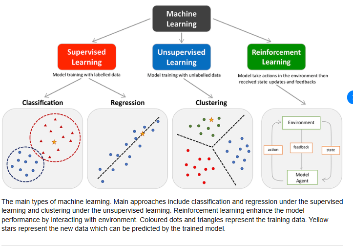
types of machine learning model [here] (https://www.google.com/search?sca_esv=5973c132c1dd70df&udm=2&fbs=AIIjpHxU7SXXniUZfeShr2fp4giZ1Y6MJ25_tmWITc7uy4KIeoJTKjrFjVxydQWqI2NcOha3O1YqG67F0QIhAO)
import numpy as np
import pandas as pd
from sklearn.model_selection import train_test_split
from sklearn.neural_network import MLPClassifier
from sklearn.metrics import classification_report, accuracy_score
import matplotlib.pyplot as plt

# Step 1: Create the dataset
data = {
    "Name": ["Dorji", "Tashi", "Pema", "Dawa", "Nima", "Karma", "Dema", "Dechen", "Kelzang", "Zam"],
    "Math": [20, 35, 70, 40, 50, 67, 88, 46, 67, 46],
    "Sci": [54, 60, 54, 34, 36, 67, 89, 90, 57, 67],
    "Eng": [67, 76, 55, 45, 34, 25, 78, 47, 67, 76],
    "Dzo": [93, 59, 76, 77, 59, 47, 29, 39, 71, 62],
    "Total": [234, 230, 255, 196, 179, 206, 284, 222, 262, 251]
}

# Convert the data to a pandas DataFrame
df = pd.DataFrame(data)

# Step 2: Convert Total score into classes (Low, Medium, High)
bins = [0, 200, 250, 300]
labels = ['Low', 'Medium', 'High']
df['Class'] = pd.cut(df['Total'], bins=bins, labels=labels)

# Step 3: Prepare the features (X) and target (y)
X = df[['Math', 'Sci', 'Eng', 'Dzo']].values  # Features
y = df['Class'].values  # Target (Class)

# Step 4: Split the data into training and testing sets
X_train, X_test, y_train, y_test = train_test_split(X, y, test_size=0.3, random_state=42)

# Step 5: Initialize the classifier (MLPClassifier)
classifier = MLPClassifier(hidden_layer_sizes=(10,), activation='relu', solver='adam', max_iter=1000, random_state=42)

# Step 6: Train the model
classifier.fit(X_train, y_train)

# Step 7: Evaluate the model
y_pred = classifier.predict(X_test)

# Print classification report and accuracy
print(f"Accuracy: {accuracy_score(y_test, y_pred):.2f}")
print("Classification Report:")
print(classification_report(y_test, y_pred))

# Step 8: Visualize some predictions
fig, axs = plt.subplots(1, 5, figsize=(15, 3))
for i in range(5):
    axs[i].bar(['Predicted', 'Actual'], [y_pred[i], y_test[i]], color=['blue', 'red'])
    axs[i].set_title(f"Student {i+1}")
    axs[i].set_ylim([0, 1])
plt.tight_layout()
plt.show()
import numpy as np
import pandas as pd
from sklearn.model_selection import train_test_split
from sklearn.neural_network import MLPClassifier
from sklearn.metrics import classification_report, accuracy_score
import matplotlib.pyplot as plt

# Step 1: Create the dataset
data = {
    "Name": ["Dorji", "Tashi", "Pema", "Dawa", "Nima", "Karma", "Dema", "Dechen", "Kelzang", "Zam"],
    "Math": [20, 35, 70, 40, 50, 67, 88, 46, 67, 46],
    "Sci": [54, 60, 54, 34, 36, 67, 89, 90, 57, 67],
    "Eng": [67, 76, 55, 45, 34, 25, 78, 47, 67, 76],
    "Dzo": [93, 59, 76, 77, 59, 47, 29, 39, 71, 62],
    "Total": [234, 230, 255, 196, 179, 206, 284, 222, 262, 251]
}
import numpy as np
import pandas as pd
from sklearn.model_selection import train_test_split
from sklearn.neural_network import MLPClassifier
from sklearn.metrics import classification_report, accuracy_score
import matplotlib.pyplot as plt

# Step 1: Create the dataset
data = {
    "Name": ["Dorji", "Tashi", "Pema", "Dawa", "Nima", "Karma", "Dema", "Dechen", "Kelzang", "Zam"],
    "Math": [20, 35, 70, 40, 50, 67, 88, 46, 67, 46],
    "Sci": [54, 60, 54, 34, 36, 67, 89, 90, 57, 67],
    "Eng": [67, 76, 55, 45, 34, 25, 78, 47, 67, 76],
    "Dzo": [93, 59, 76, 77, 59, 47, 29, 39, 71, 62],
    "Total": [234, 230, 255, 196, 179, 206, 284, 222, 262, 251]
  Cell In[19], line 85
    "Total": [234, 230, 255, 196, 179, 206, 284, 222, 262, 251]
                                                               ^
_IncompleteInputError: incomplete input
import numpy as np
import pandas as pd
from sklearn.model_selection import train_test_split
from sklearn.linear_model import LinearRegression
from sklearn.metrics import mean_squared_error, r2_score
import matplotlib.pyplot as plt

# Create the dataset
data = {
    "Name": ["Dorji", "Tashi", "Pema", "Dawa", "Nima", "Karma", "Dema", "Dechen", "Kelzang", "Zam"],
    "Math": [20, 35, 70, 40, 50, 67, 88, 46, 67, 46],
    "Sci": [54, 60, 54, 34, 36, 67, 89, 90, 57, 67],
    "Eng": [67, 76, 55, 45, 34, 25, 78, 47, 67, 76],
    "Dzo": [93, 59, 76, 77, 59, 47, 29, 39, 71, 62],
    "Total": [234, 230, 255, 196, 179, 206, 284, 222, 262, 251]
}

# Convert the data to a pandas DataFrame
df = pd.DataFrame(data)

# Prepare the features (X) and target (y)
X = df[['Math', 'Sci', 'Eng', 'Dzo']].values  # Features
y = df['Total'].values  # Target (Total)

# Step 2: Split the data into training and testing sets
X_train, X_test, y_train, y_test = train_test_split(X, y, test_size=0.3, random_state=42)

# Step 3: Initialize the Linear Regression model
regressor = LinearRegression()

# Step 4: Train the model
regressor.fit(X_train, y_train)

# Step 5: Make predictions on the test set
y_pred = regressor.predict(X_test)

# Step 6: Evaluate the model
mse = mean_squared_error(y_test, y_pred)
r2 = r2_score(y_test, y_pred)

print(f"Mean Squared Error: {mse:.2f}")
print(f"R2 Score: {r2:.2f}")

# Step 7: Plot predictions vs actual
plt.figure(figsize=(8, 5))
plt.scatter(y_test, y_pred)
plt.plot([min(y_test), max(y_test)], [min(y_test), max(y_test)], color='red', linestyle='--')  # Ideal line
plt.xlabel('Actual Total')
plt.ylabel('Predicted Total')
plt.title('Actual vs Predicted Total')
plt.show()
Mean Squared Error: 0.00
R2 Score: 1.00

import numpy as np
import pandas as pd
from sklearn.cluster import KMeans
import matplotlib.pyplot as plt

# Create the dataset
data = {
    "Name": ["Dorji", "Tashi", "Pema", "Dawa", "Nima", "Karma", "Dema", "Dechen", "Kelzang", "Zam"],
    "Math": [20, 35, 70, 40, 50, 67, 88, 46, 67, 46],
    "Sci": [54, 60, 54, 34, 36, 67, 89, 90, 57, 67],
    "Eng": [67, 76, 55, 45, 34, 25, 78, 47, 67, 76],
    "Dzo": [93, 59, 76, 77, 59, 47, 29, 39, 71, 62],
    "Total": [234, 230, 255, 196, 179, 206, 284, 222, 262, 251]
}

# Convert the data to a pandas DataFrame
df = pd.DataFrame(data)

# Prepare the features (X)
X = df[['Math', 'Sci', 'Eng', 'Dzo']].values  # Features (no target for clustering)

# Step 1: Apply KMeans clustering
kmeans = KMeans(n_clusters=3, random_state=42)  # We will assume 3 clusters
kmeans.fit(X)

# Step 2: Assign the predicted clusters to the DataFrame
df['Cluster'] = kmeans.labels_

# Step 3: Print the cluster assignments
print("\nCluster assignments for each student:")
print(df[['Name', 'Cluster']])

# Step 4: Visualize the clustering (2D scatter plot for simplicity)
plt.figure(figsize=(8, 5))

# Plot based on first two features (Math and Sci)
plt.scatter(df['Math'], df['Sci'], c=df['Cluster'], cmap='viridis')
plt.xlabel('Math')
plt.ylabel('Sci')
plt.title('K-Means Clustering (Math vs Sci)')
plt.colorbar(label='Cluster')
plt.show()
Cluster assignments for each student:
      Name  Cluster
0    Dorji        0
1    Tashi        1
2     Pema        2
3     Dawa        0
4     Nima        0
5    Karma        2
6     Dema        1
7   Dechen        1
8  Kelzang        2
9      Zam        1

Explanation of the Clustering Code:
Data Setup: We use the same dataset as before, but this time only the features (Math, Sci, Eng, and Dzo) are used for clustering.
K-Means Clustering: We apply K-Means with 3 clusters (n_clusters=3) to group the students based on their features.
Cluster Assignment: The cluster labels assigned by K-Means are added to the DataFrame.
Visualization: A scatter plot is created to visualize the clusters based on two features: Math and Sci. Each point is colored according to its assigned cluster.
import numpy as np
import pandas as pd
from sklearn.preprocessing import StandardScaler
from sklearn.cluster import KMeans
import matplotlib.pyplot as plt
from sklearn.decomposition import PCA

# Data given
data = {
    "Name": ["Dorji", "Tashi", "Pema", "Dawa", "Nima", "Karma", "Dema", "Dechen", "Kelzang", "Zam"],
    "Math": [20, 35, 70, 40, 50, 67, 88, 46, 67, 46],
    "Sci": [54, 60, 54, 34, 36, 67, 89, 90, 57, 67],
    "Eng": [67, 76, 55, 45, 34, 25, 78, 47, 67, 76],
    "Dzo": [93, 59, 76, 77, 59, 47, 29, 39, 71, 62],
    "Total": [234, 230, 255, 196, 179, 206, 284, 222, 262, 251]
}

# Create a DataFrame
df = pd.DataFrame(data)

# Extract the features (subjects) for clustering
features = df[["Math", "Sci", "Eng", "Dzo"]]

# Standardize the data
scaler = StandardScaler()
scaled_features = scaler.fit_transform(features)

# Apply KMeans clustering (we can try 3 clusters, but you can adjust as needed)
kmeans = KMeans(n_clusters=3, random_state=42)
df['Cluster'] = kmeans.fit_predict(scaled_features)

# Add the cluster information to the DataFrame
print(df[['Name', 'Cluster']])

# Visualize the clusters using PCA (2D reduction for simplicity)
pca = PCA(n_components=2)
reduced_features = pca.fit_transform(scaled_features)

# Plot the clusters
plt.figure(figsize=(8, 6))
plt.scatter(reduced_features[:, 0], reduced_features[:, 1], c=df['Cluster'], cmap='viridis', s=100)
for i, name in enumerate(df['Name']):
    plt.annotate(name, (reduced_features[i, 0], reduced_features[i, 1]), fontsize=9)
plt.title('PCA Projection of Clusters')
plt.xlabel('PCA 1')
plt.ylabel('PCA 2')
plt.colorbar(label='Cluster')
plt.show()
      Name  Cluster
0    Dorji        0
1    Tashi        1
2     Pema        2
3     Dawa        0
4     Nima        0
5    Karma        2
6     Dema        1
7   Dechen        1
8  Kelzang        2
9      Zam        1

import pandas as pd
import numpy as np
from sklearn.model_selection import train_test_split
from sklearn.preprocessing import StandardScaler
from sklearn.neural_network import MLPRegressor
from sklearn.metrics import mean_absolute_error

# Dataset
data = {
    "Math": [20,35,70,40,50,67,88,46,67,46],
    "Sci": [54,60,54,34,36,67,89,90,57,67],
    "Eng": [67,76,55,45,34,25,78,47,67,76],
    "Dzo": [93,59,76,77,59,47,29,39,71,62],
    "Total": [234,230,255,196,179,206,284,222,262,251]
}

df = pd.DataFrame(data)

X = df[["Math", "Sci", "Eng", "Dzo"]]
y = df[["Total"]]   # keep as 2D for scaling

# Train-test split
X_train, X_test, y_train, y_test = train_test_split(
    X, y, test_size=0.2, random_state=42
)

# Scale X
X_scaler = StandardScaler()
X_train = X_scaler.fit_transform(X_train)
X_test = X_scaler.transform(X_test)

# Scale y
y_scaler = StandardScaler()
y_train = y_scaler.fit_transform(y_train)
y_test_scaled = y_scaler.transform(y_test)

# Neural Network Model
model = MLPRegressor(
    hidden_layer_sizes=(16, 8),
    activation='relu',
    max_iter=5000,
    random_state=42
)

# Train
model.fit(X_train, y_train.ravel())

# Predict (scaled)
y_pred_scaled = model.predict(X_test)

# Inverse transform predictions
y_pred = y_scaler.inverse_transform(y_pred_scaled.reshape(-1, 1))

# Evaluation
print("Actual:", y_test.values.flatten())
print("Predicted:", y_pred.flatten())
print("Mean Absolute Error:", mean_absolute_error(y_test, y_pred))
Actual: [262 230]
Predicted: [259.80699632 240.12737015]
Mean Absolute Error: 6.160186915217977