Session 4: Data Science: Machine Learning
Attending the Data Science Fitting class was not as I had expected, as the lessons involved many mathematical concepts and coding. I will try to keep track of my learning experiences with the help of my colleagues and online resources.
Attending help session from Mr. Jean Michel Molennar

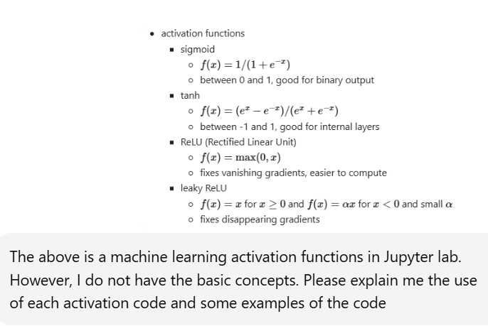
I used Chatgpt to understand the machine learning functions in details. The following are the prompt used for learning.
Sigmoid
import numpy as np
def sigmoid(x): return 1 / (1 + np.exp(-x))
x = np.array([-2, -1, 0, 1, 2]) print(sigmoid(x))
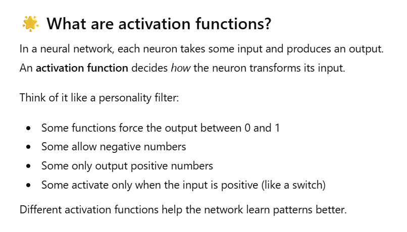
Tanh Activation
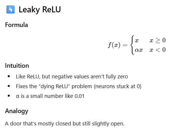
Leaky ReLU
Future Predictions of Fire counts
In [2]:
import pandas as pd

# Load dataset
df = pd.read_csv("datasets/firecounts.csv")

# View first rows
print(df.head())

# Summary statistics
print(df.describe())
   Year  Fire Counts
0  2001          199
1  2002          127
2  2003          170
3  2004          219
4  2005          204
              Year  Fire Counts
count    24.000000    24.000000
mean   2012.500000   240.125000
std       7.071068    95.406823
min    2001.000000    97.000000
25%    2006.750000   169.750000
50%    2012.500000   226.000000
75%    2018.250000   282.750000
max    2024.000000   442.000000
Counts Predictions based on Year.
In [4]:
import numpy as np
from sklearn.model_selection import train_test_split

X = df[["Year"]]      # Feature
y = df["Fire Counts"] # Target

X_train, X_test, y_train, y_test = train_test_split(
    X, y, test_size=0.2, random_state=42
)
Linear Regression
In [7]:
from sklearn.linear_model import LinearRegression

model = LinearRegression()
model.fit(X_train, y_train)

print("Model trained.")
print("Coefficient:", model.coef_)
print("Intercept:", model.intercept_)
Model trained.
Coefficient: [-3.01486698]
Intercept: 6300.923317683881
Forecast Future years (2025-2030)
In [8]:
future_years = pd.DataFrame({"Year": np.arange(2025, 2031)})
future_predictions = model.predict(future_years)

forecast_df = pd.DataFrame({
    "Year": future_years["Year"],
    "Predicted Fire Counts": future_predictions
})

print(forecast_df)
   Year  Predicted Fire Counts
0  2025             195.817684
1  2026             192.802817
2  2027             189.787950
3  2028             186.773083
4  2029             183.758216
5  2030             180.743349
Historical vs Forecast
In [9]:
plt.figure(figsize=(10,5))

# Plot historical data
plt.plot(df["Year"], df["Fire Counts"], marker='o', label="Historical Data")

# Plot forecast
plt.plot(forecast_df["Year"], forecast_df["Predicted Fire Counts"],
         marker='x', linestyle="--", label="Forecast")

plt.xlabel("Year")
plt.ylabel("Fire Counts")
plt.title("Historical and Forecasted Fire Counts")
plt.legend()
plt.grid(True)
plt.show()

Image visualization
In [ ]:
I used Chatgpt promt to visualize the original image in different colors and sizes.
Original Image

In [18]:
from PIL import Image, ImageOps, ImageFilter
import numpy as np
import matplotlib.pyplot as plt

# Load image
img = Image.open("images/dzo.png").convert("RGBA")

# Convert to grayscale for masking
gray = ImageOps.grayscale(img)

# --- BETTER MASK ---
# 1. Lower threshold to catch faint lines (light blue)
# 2. Invert mask so lines become white (255)
mask = gray.point(lambda x: 255 if x < 230 else 0, mode="L")

# --- THICKEN LINES ---
# Apply dilation using a blur + threshold trick
mask = mask.filter(ImageFilter.GaussianBlur(1.2))     # smooth + thicken
mask = mask.point(lambda x: 255 if x > 30 else 0, 'L') # restore clean mask

# Function to recolor the CLEAN mask
def color_line(mask, color):
    w, h = mask.size
    out = Image.new("RGBA", (w, h), color=color)
    out.putalpha(mask)  # treat mask as alpha channel
    return out

# Create colored lines
red_line    = color_line(mask, (255, 0, 0, 255))
yellow_line = color_line(mask, (255, 255, 0, 255))
blue_line   = color_line(mask, (0, 0, 255, 255))

# Display
plt.figure(figsize=(12, 4))

plt.subplot(1, 3, 1)
plt.imshow(red_line)
plt.title("Red Line")
plt.axis("off")

plt.subplot(1, 3, 2)
plt.imshow(yellow_line)
plt.title("Yellow Line")
plt.axis("off")

plt.subplot(1, 3, 3)
plt.imshow(blue_line)
plt.title("Blue Line")
plt.axis("off")

plt.show()
