[Kelzang Wangdi] - Fab Futures - Data Science

Home About

Presentation

While working on my assignments, I utilized the Python codes provided in the class folders as a foundational reference to understand the methods and procedures. To deepen my comprehension of the logic behind the codes and to assist in writing parts of my own scripts, I consulted AI-based tools, particularly ChatGPT (OpenAI, 2023), which provided explanations, step-by-step clarifications, and guidance on implementing functions effectively. Additionally, I referred to Grokai and Genome platforms for minor clarifications and supplementary examples. All external assistance was used strictly to enhance my understanding and support my learning process; I ensured that the final work submitted is my own, and these sources have been properly acknowledged to maintain academic integrity.

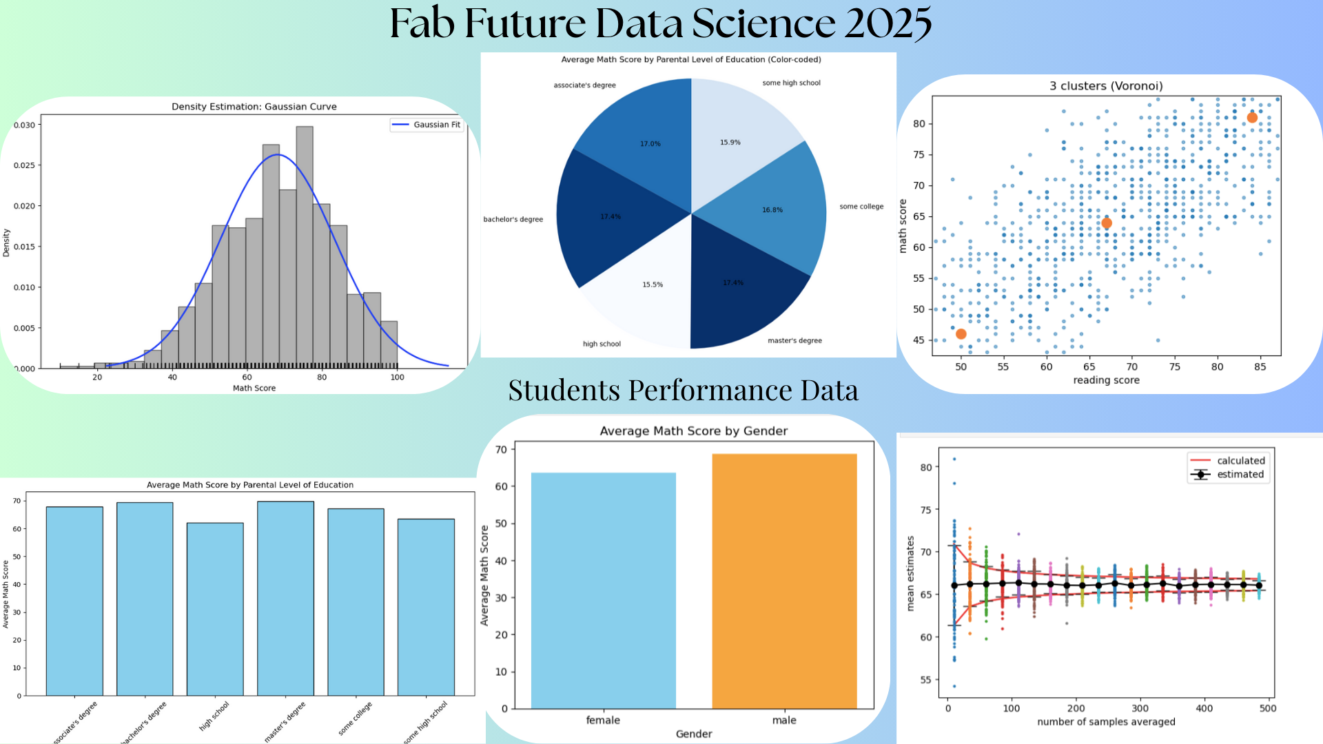
Presentation Slide

from IPython.display import HTML
HTML('<img src="images/presentation.png" width="900">')

Week 01

Introduction to Data Science

The course began with an introduction to data science, where I learned how data is collected, processed, analyzed, and interpreted to support decision-making. I was introduced to key concepts such as datasets, variables, data types, and basic data analysis workflows. This topic helped me understand the importance of data in today’s digital world and how data science is applied across various fields such as education, health, engineering, and social sciences. It also laid a strong foundation for using programming tools to extract meaningful insights from raw data.

Fab Labs

I was introduced to the concept of Fab Labs (Fabrication Laboratories) and their role in innovation, digital fabrication, and hands-on learning. Fab Labs provide access to modern tools such as 3D printers, laser cutters, CNC machines, and electronics workstations, enabling learners to turn ideas into physical prototypes. This topic helped me understand how Fab Labs promote creativity, problem-solving, and collaboration while supporting local and global innovation networks. It also highlighted how Fab Labs connect technology, design, and data-driven thinking.

21st-Century Vocational Skills

The course emphasized the importance of 21st-century vocational skills, including digital literacy, critical thinking, collaboration, creativity, and adaptability. I learned how technical skills such as coding and data analysis must be combined with soft skills like communication and teamwork to succeed in modern workplaces. This topic helped me recognize the value of lifelong learning and the need to continuously update skills in response to technological advancements.

Selecting Datasets from Open Sources

I learned how to identify and select appropriate datasets from open-source platforms for data analysis projects. This included understanding data relevance, quality, structure, and ethical considerations such as data privacy and proper attribution. Exploring open-source datasets helped me gain practical experience in working with real-world data and improved my ability to choose datasets that align with specific research questions or project goals.

Introduction to the JupyterLab Interface

The course also introduced me to the JupyterLab interface, which is a powerful environment for data science and programming. I learned how to create and manage notebooks, write and execute Python code, add markdown text for documentation, and visualize data using plots and charts. This topic helped me understand how JupyterLab supports interactive learning, experimentation, and reproducible research, making it an essential tool for data analysis and collaborative work.

Dataset for this course

For this course, I have decided to use the Dataset on "School Performance Analysis" of the US DEPARTMENT OF EDUCATION: College Scorecard [https://collegescorecard.ed.gov/data] This data talks about how gender, parental education, and preparation affect exam results.

Tools

In this lesson on tools, I learned how Pandas, NumPy, and Matplotlib work together as core Python libraries for data science.

NumPy

Numpy was introduced as the foundation for numerical computing, enabling efficient handling of arrays, mathematical operations, and large datasets. Through NumPy, I learned how to perform calculations, manipulate numerical data, and work with multidimensional arrays, which are essential for data processing and scientific computing.

Pandas

Pandas was presented as a powerful library for data manipulation and analysis. I learned how to load datasets from CSV and other file formats, explore data using dataframes, clean and preprocess data, handle missing values, and perform operations such as filtering, grouping, and aggregation. Pandas helped me understand how to organize and analyze structured data in a clear and efficient manner, making it easier to extract insights and prepare data for further analysis.

Matplotlib

Matplotlib was introduced as a visualization tool for presenting data in a meaningful way. I learned how to create various types of plots such as line graphs, bar charts, histograms, and scatter plots to visualize trends and patterns in data. Using Matplotlib helped me understand how visual representation of data supports better interpretation and communication of results. Together, Pandas, NumPy, and Matplotlib formed a complete workflow for data analysis, from data loading and processing to visualization and interpretation.

Assignment (Data Visualization using tools)

In this work, I used Pandas, NumPy, and Matplotlib to complete the full data analysis process, starting from data cleaning to data visualization. Pandas helped me load and explore the dataset, clean missing or inconsistent values, filter and organize the data, and prepare it for analysis. NumPy supported efficient numerical operations and transformations, enabling me to handle calculations and improve performance when working with numerical data. Finally, I used Matplotlib to visualize the cleaned data through charts and graphs such as bar plots, line graphs, and histograms, which helped me identify patterns, trends, and insights and communicate the results clearly and effectively.

Example

import pandas as pd
import numpy as np
from matplotlib import pyplot as plt
data = pd.read_csv("~/work/kelzang-wangdi/datasets/StudentsPerformance.csv")
data

	gender	race/ethnicity	parental level of education	lunch	test preparation course	math score	reading score	writing score
0	female	group B	bachelor's degree	standard	none	72	72	74
1	female	group C	some college	standard	completed	69	90	88
2	female	group B	master's degree	standard	none	90	95	93
3	male	group A	associate's degree	free/reduced	none	47	57	44
4	male	group C	some college	standard	none	76	78	75
...	...	...	...	...	...	...	...	...
995	female	group E	master's degree	standard	completed	88	99	95
996	male	group C	high school	free/reduced	none	62	55	55
997	female	group C	high school	free/reduced	completed	59	71	65
998	female	group D	some college	standard	completed	68	78	77
999	female	group D	some college	free/reduced	none	77	86	86

1000 rows × 8 columns

Show first and last five Data

data.head()

	gender	race/ethnicity	parental level of education	lunch	test preparation course	math score	reading score	writing score
0	female	group B	bachelor's degree	standard	none	72	72	74
1	female	group C	some college	standard	completed	69	90	88
2	female	group B	master's degree	standard	none	90	95	93
3	male	group A	associate's degree	free/reduced	none	47	57	44
4	male	group C	some college	standard	none	76	78	75

data.tail()

	gender	race/ethnicity	parental level of education	lunch	test preparation course	math score	reading score	writing score
995	female	group E	master's degree	standard	completed	88	99	95
996	male	group C	high school	free/reduced	none	62	55	55
997	female	group C	high school	free/reduced	completed	59	71	65
998	female	group D	some college	standard	completed	68	78	77
999	female	group D	some college	free/reduced	none	77	86	86

Descriptive statistics

data.describe()

	math score	reading score	writing score
count	1000.00000	1000.000000	1000.000000
mean	66.08900	69.169000	68.054000
std	15.16308	14.600192	15.195657
min	0.00000	17.000000	10.000000
25%	57.00000	59.000000	57.750000
50%	66.00000	70.000000	69.000000
75%	77.00000	79.000000	79.000000
max	100.00000	100.000000	100.000000

To show column names

data.columns

Index(['gender', 'race/ethnicity', 'parental level of education', 'lunch',
       'test preparation course', 'math score', 'reading score',
       'writing score'],
      dtype='object')

Data Information

data.info()

<class 'pandas.core.frame.DataFrame'>
RangeIndex: 1000 entries, 0 to 999
Data columns (total 8 columns):
 #   Column                       Non-Null Count  Dtype 
---  ------                       --------------  ----- 
 0   gender                       1000 non-null   object
 1   race/ethnicity               1000 non-null   object
 2   parental level of education  1000 non-null   object
 3   lunch                        1000 non-null   object
 4   test preparation course      1000 non-null   object
 5   math score                   1000 non-null   int64 
 6   reading score                1000 non-null   int64 
 7   writing score                1000 non-null   int64 
dtypes: int64(3), object(5)
memory usage: 62.6+ KB

Find Missing Values

data.isnull()

	gender	race/ethnicity	parental level of education	lunch	test preparation course	math score	reading score	writing score
0	False	False	False	False	False	False	False	False
1	False	False	False	False	False	False	False	False
2	False	False	False	False	False	False	False	False
3	False	False	False	False	False	False	False	False
4	False	False	False	False	False	False	False	False
...	...	...	...	...	...	...	...	...
995	False	False	False	False	False	False	False	False
996	False	False	False	False	False	False	False	False
997	False	False	False	False	False	False	False	False
998	False	False	False	False	False	False	False	False
999	False	False	False	False	False	False	False	False

1000 rows × 8 columns

Data Visualization

import matplotlib.pyplot as plt

genders = data['gender'].unique() 
for g in genders:
    subset = data[data['gender'] == g]  
    plt.scatter(subset['reading score'], subset['writing score'], label=g)

plt.xlabel('Reading Score')
plt.ylabel('Writing Score')
plt.title('Male and Female (Writing Score Vs Reading Score')
plt.legend()
plt.show()

Week 02

Function Fitting

In this lesson, I learned how mathematical functions can be fitted to data in order to model relationships between variables and make predictions. I began by understanding the role of variables, distinguishing between independent and dependent variables, and how linear and quadratic models can be used to represent real-world trends. I explored function fitting techniques using polynomial models, particularly linear and quadratic functions, and learned how the:

polyfit routine

The polyfit routine is used to find the best-fitting polynomial coefficients for a given dataset. The lesson also introduced the underlying algorithm of:

Singular Value Decomposition (SVD),

Singular Value Decomposition (SVD), which helps solve least-squares problems in a stable and efficient way, especially when data is noisy or nearly dependent. I further learned how to use the:

lstsq routine

lstsq routine to compute least-squares solutions for over-determined systems and the least_squares routine for more flexible and advanced optimization of model parameters. Finally, I was introduced to the concept of regularization, which helps prevent overfitting by adding constraints to the model, improving its ability to generalize to new data. Together, these topics strengthened my understanding of how mathematical modeling and numerical methods are applied to real data analysis problems.

Assignment

import numpy as np
import pandas as pd
import matplotlib.pyplot as plt

df = pd.read_csv("~/work/kelzang-wangdi/datasets/StudentsPerformance.csv")  
x_column = 'writing score'   
y_column = 'math score'      

x = df[x_column].dropna().values
y = df[y_column].dropna().values

np.set_printoptions(precision=3)

coeff1 = np.polyfit(x, y, 1)
pfit1 = np.poly1d(coeff1)

coeff2 = np.polyfit(x, y, 2)
pfit2 = np.poly1d(coeff2)

xfit = np.linspace(np.min(x), np.max(x), 100)
yfit1 = pfit1(xfit)
yfit2 = pfit2(xfit)

print(f"first-order fit coefficients: {coeff1}")
print(f"second-order fit coefficients: {coeff2}")

plt.figure(figsize=(8,6))
plt.plot(x, y, 'o', alpha=0.6, label='data')
plt.plot(xfit, yfit1, 'g-', label='linear fit')
plt.plot(xfit, yfit2, 'r-', label='quadratic fit')
plt.xlabel(x_column)
plt.ylabel(y_column)
plt.title(f"Polynomial Fit: {y_column} vs {x_column}")
plt.legend()
plt.show()

first-order fit coefficients: [ 0.801 11.583]
second-order fit coefficients: [-1.238e-03  9.640e-01  6.503e+00]

Machine Learning

Different Functions

 1. Sigmoid
 2. Tanh
 3. ReLU
 4. Leaky ReLU

These functions help neural networks learn complex patterns by introducing non-linearity.

Scikit Learn Library for Machin Learning

The Scikit-learn library provides a unified and easy-to-use platform for implementing a wide range of machine learning algorithms in Python, making it accessible to both beginners and experienced users. It offers consistent APIs for tasks such as data preprocessing, classification, regression, clustering, dimensionality reduction, and model evaluation, which simplifies the entire machine learning workflow. By integrating seamlessly with libraries like NumPy, Pandas, and Matplotlib, Scikit-learn allows users to efficiently prepare data, train models, tune parameters, and assess performance using well-documented and reliable tools. This consistency and simplicity enable faster experimentation, reproducibility, and practical application of machine learning techniques to real-world problems.

import pandas as pd
import numpy as np
from sklearn.model_selection import train_test_split
from sklearn.preprocessing import StandardScaler
from sklearn.neural_network import MLPRegressor
from sklearn.metrics import mean_squared_error, r2_score
import matplotlib.pyplot as plt

df = pd.read_csv("~/work/kelzang-wangdi/datasets/StudentsPerformance.csv")  
feature_cols = ['math score', 'reading score']  
target_col = 'writing score'                    

X = df[feature_cols].values
y = df[target_col].values

X_train, X_test, y_train, y_test = train_test_split(X, y, test_size=0.2, random_state=42)

scaler = StandardScaler()
X_train = scaler.fit_transform(X_train)
X_test = scaler.transform(X_test)

model = MLPRegressor(hidden_layer_sizes=(50,50),
                     activation='tanh',
                     solver='adam',
                     max_iter=1000,
                     random_state=42)

model.fit(X_train, y_train)

y_pred = model.predict(X_test)

mse = mean_squared_error(y_test, y_pred)
r2 = r2_score(y_test, y_pred)

print(f"Mean Squared Error: {mse:.3f}")
print(f"R2 Score: {r2:.3f}")

plt.figure(figsize=(8,6))
plt.scatter(y_test, y_pred, alpha=0.6)
plt.xlabel("True Writing Score")
plt.ylabel("Predicted Writing Score")
plt.title("MLP Regressor Predictions with Tanh Activation")
plt.plot([y_test.min(), y_test.max()], [y_test.min(), y_test.max()], 'r--', lw=2)  
plt.show()

Mean Squared Error: 26.222
R2 Score: 0.891

/opt/conda/lib/python3.13/site-packages/sklearn/neural_network/_multilayer_perceptron.py:781: ConvergenceWarning: Stochastic Optimizer: Maximum iterations (1000) reached and the optimization hasn't converged yet.
  warnings.warn(

Functions

import numpy as np
import pandas as pd
import matplotlib.pyplot as plt

data = pd.read_csv("~/work/kelzang-wangdi/datasets/StudentsPerformance.csv")

x = data['writing score'].values

x = np.sort(x)

plt.plot(x, 1/(1+np.exp(-x)), label='Sigmoid')
plt.plot(x, np.tanh(x), label='Tanh')
plt.plot(x, np.where(x < 0, 0, x), label='ReLU')
plt.plot(x, np.where(x < 0, 0.1*x, x), '--', label='Leaky ReLU')

plt.legend()
plt.xlabel("Input values (from your data)")
plt.ylabel("Activation output")
plt.title("Activation Functions using Uploaded Data")
plt.show()

Probabilty

Definition

Probability is a branch of mathematics that deals with measuring the likelihood of events occurring, expressed as a value between 0 and 1. It provides a systematic way to quantify uncertainty and make informed predictions based on available data. In simple terms, probability helps answer questions such as how likely an outcome is to happen and how confident we can be in a particular result.

Probability in Data Science

In data science, probability plays a fundamental role in analyzing data and making decisions under uncertainty. It is used in statistical modeling, hypothesis testing, and predictive analytics to estimate future outcomes based on historical data. Probability forms the basis of many machine learning algorithms, such as Naive Bayes classifiers, probabilistic graphical models, and Bayesian inference. It also helps in understanding data distributions, measuring risk, handling randomness and noise in data, and evaluating model performance. Overall, probability enables data scientists to draw reliable conclusions, make predictions, and build models that can generalize well to real-world situations.

Histogram

import pandas as pd
import numpy as np
import matplotlib.pyplot as plt

data = pd.read_csv("~/work/kelzang-wangdi/datasets/StudentsPerformance.csv")

scores = data['math score']

# Plot histogram (normalized)
plt.hist(scores, bins=20, density=True, alpha=0.6)

mean = scores.mean()
std = scores.std()

x = np.linspace(scores.min(), scores.max(), 200)
gaussian = (1 / (std * np.sqrt(2 * np.pi))) * np.exp(-0.5 * ((x - mean) / std) ** 2)

plt.plot(x, gaussian)

plt.xlabel("Math Score")
plt.ylabel("Density")
plt.title("Histogram of Math Scores with Gaussian Curve")

plt.show()

Averaging

Averaging in probability refers to the process of finding the expected or mean value of a random variable by considering all possible outcomes and their probabilities. Instead of simply taking a regular arithmetic average of observed values, probabilistic averaging weights each outcome by how likely it is to occur. This gives a more accurate representation of what we expect to happen over many repeated trials. In probability and data science, this concept is known as the expected value. It is calculated by multiplying each possible outcome by its probability and then summing these products. Averaging in probability is widely used to summarize uncertain situations, evaluate risks, compare outcomes, and support decision-making. For example, in data science and machine learning, probabilistic averaging helps estimate model predictions, reduce noise through repeated sampling, and understand long-term behavior of random processes.

import numpy as np
import pandas as pd
import matplotlib.pyplot as plt

data = pd.read_csv("~/work/kelzang-wangdi/datasets/StudentsPerformance.csv")  
column = "math score"             
x = data[column].dropna().values

true_mean = np.mean(x)
true_std = np.std(x)

trials = 200
points = np.arange(10, 500, 25)
means = np.zeros((trials, len(points)))

for p in range(len(points)):
    N = points[p]
    for t in range(trials):
        sample = np.random.choice(x, size=N, replace=True)
        means[t, p] = np.mean(sample)

plt.plot(points, true_mean + true_std / np.sqrt(points), 'r', label='calculated')
plt.plot(points, true_mean - true_std / np.sqrt(points), 'r')

estimated_mean = np.mean(means, axis=0)
estimated_std = np.std(means, axis=0)

plt.errorbar(points, estimated_mean, yerr=estimated_std,
             fmt='k-o', capsize=7, label='estimated')

for p in range(len(points)):
    plt.plot(np.full(trials, points[p]), means[:, p], 'o', markersize=2)

plt.xlabel('number of samples averaged')
plt.ylabel('mean estimates')
plt.legend()
plt.show()

Explanation

This graph illustrates the concept of the Central Limit Theorem and the reduction of uncertainty through averaging. The horizontal axis represents the number of samples averaged (the sample size, ), and the vertical axis shows the resulting mean estimates from multiple simulations or experiments. The individual colored dots represent the many different mean estimates obtained for each sample size. The black line with error bars (labeled "estimated") shows the sample mean of these estimates and their standard deviation (the error bars) at each . The red line (labeled "calculated") represents the theoretical population mean (the true value) and the theoretical standard error ( ), showing how the expected range of sample means shrinks as increases. As the number of samples averaged increases, the spread of the individual mean estimates (the dots) decreases, and both the estimated and calculated uncertainty bands narrow, demonstrating that a larger sample size leads to more consistent and precise estimates that converge toward the true population mean.

Density Estimation

Density estimation in data science is the process of estimating the underlying probability distribution of a dataset based on observed data points. Instead of assuming that data follows a known distribution, density estimation helps describe how data values are spread across the range of possible values. The result is a probability density function (PDF) that shows where data points are concentrated and how likely different values are to occur. In data science, density estimation is used to understand data distributions, detect patterns, and identify anomalies or outliers. Common methods include parametric approaches, such as assuming a normal (Gaussian) distribution and estimating its parameters (mean and variance), and non-parametric approaches, such as kernel density estimation (KDE), which makes fewer assumptions about the data’s shape. Density estimation is important in tasks like data visualization, probabilistic modeling, clustering, anomaly detection, and feature analysis, as it provides a foundation for making probabilistic inferences from data.

Voronoi Cluster, K-Means, Elbow Plot

%matplotlib inline
import numpy as np
import pandas as pd
import matplotlib.pyplot as plt
from scipy.spatial import Voronoi, voronoi_plot_2d

data = pd.read_csv("~/work/kelzang-wangdi/datasets/StudentsPerformance.csv") 
xcol = "reading score"  
ycol = "math score"  

x = data[xcol].dropna().values
y = data[ycol].dropna().values

N = min(len(x), len(y))
x = x[:N]
y = y[:N]

nsteps = 1000
momentum = 0.  

def kmeans(x, y, momentum, nclusters):
    indices = np.random.uniform(low=0, high=len(x), size=nclusters).astype(int)
    mux = x[indices]
    muy = y[indices]

    for _ in range(nsteps):
        X = np.outer(x, np.ones(len(mux)))
        Y = np.outer(y, np.ones(len(muy)))
        Mux = np.outer(np.ones(len(x)), mux)
        Muy = np.outer(np.ones(len(x)), muy)

        distances = np.sqrt((X - Mux)**2 + (Y - Muy)**2)
        mins = np.argmin(distances, axis=1)

        for i in range(len(mux)):
            index = np.where(mins == i)
            if len(index[0]) > 0:
                mux[i] = np.mean(x[index])
                muy[i] = np.mean(y[index])

    distances = 0
    for i in range(len(mux)):
        index = np.where(mins == i)
        distances += np.sum(np.sqrt((x[index] - mux[i])**2 + (y[index] - muy[i])**2))

    return mux, muy, distances

def plot_kmeans(x, y, mux, muy):
    fig, ax = plt.subplots()
    ax.plot(x, y, ".", alpha=0.5)
    ax.plot(mux, muy, "r.", markersize=20)
    ax.set_xlabel(xcol)
    ax.set_ylabel(ycol)
    ax.set_title(f"{len(mux)} clusters (centroids)")
    plt.show()

def plot_Voronoi(x, y, mux, muy):
    fig, ax = plt.subplots()
    ax.plot(x, y, ".", alpha=0.5)
    vor = Voronoi(np.stack((mux, muy), axis=1))
    voronoi_plot_2d(vor, ax=ax, show_points=True, show_vertices=False, point_size=20)
    ax.set_xlabel(xcol)
    ax.set_ylabel(ycol)
    ax.set_title(f"{len(mux)} clusters (Voronoi)")
    plt.show()

distances = []

for k in range(1, 6):
    mux, muy, d = kmeans(x, y, momentum, k)
    distances.append(d)
    
    if k <= 2:
        plot_kmeans(x, y, mux, muy)
    else:
        plot_Voronoi(x, y, mux, muy)
plt.figure()
plt.plot(range(1, 6), distances, "o-")
plt.xlabel("Number of clusters")
plt.ylabel("Total distance to clusters")
plt.title("Elbow Plot")
plt.xticks(range(1, 6))
plt.show()

Explanation

K-Means is a popular unsupervised machine learning algorithm used for clustering data by partitioning it into K groups based on similarity, where each data point is assigned to the nearest cluster center (centroid). The resulting clusters can be visualized as Voronoi clusters, where the data space is divided into regions such that every point in a region is closer to its corresponding centroid than to any other centroid, forming Voronoi cells around each cluster center. An Elbow Plot is a diagnostic tool used to determine the optimal number of clusters in K-Means by plotting the number of clusters against the within-cluster sum of squares (inertia); the “elbow” point indicates where adding more clusters yields diminishing improvements, helping to select a balanced and meaningful value of K.

Transform

In data science, a transform refers to the process of changing or converting data from one format, scale, or representation to another to make it more suitable for analysis, modeling, or visualization. Transformations can be applied to individual variables (columns), entire datasets, or features, depending on the goal.

Principal Components Analysis (PCA)

Principal Component Analysis (PCA) is important because it simplifies complex datasets by reducing their dimensionality while preserving most of the essential information. By transforming correlated variables into a smaller set of uncorrelated components, PCA helps reveal hidden patterns, improves data visualization, and reduces noise. This makes it especially valuable for speeding up machine learning algorithms, preventing overfitting, and handling high-dimensional data more efficiently. Overall, PCA enhances both the interpretability and performance of data analysis processes.

import numpy as np
import matplotlib.pyplot as plt
import sklearn
import pandas as pd

data = pd.read_csv("~/work/kelzang-wangdi/datasets/StudentsPerformance.csv")

print("Columns available in your dataset:\n", data.columns)

y = data["parental level of education"].astype('category').cat.codes  
X = data[["math score", "reading score", "writing score"]].values

print(f"Your data shape (records, features): {X.shape}")

plt.scatter(X[:,0], X[:,1], c=y)
plt.xlabel("math score")
plt.ylabel("reading score")
plt.title("Students Performance: Two Features")
plt.colorbar(label="parental level of education")
plt.show()

X = X - np.mean(X, axis=0)
std = np.std(X, axis=0)
Xscale = X / np.where(std > 0, std, 1)

pca = sklearn.decomposition.PCA(n_components=3)
Xpca = pca.fit_transform(Xscale)

plt.plot(pca.explained_variance_, 'o')
plt.xlabel("component")
plt.ylabel("explained variance")
plt.show()

plt.scatter(Xpca[:,0], Xpca[:,1], c=y)
plt.xlabel("PC1")
plt.ylabel("PC2")
plt.title("PCA of Student Performance")
plt.colorbar(label="parental level of education")
plt.show()

Columns available in your dataset:
 Index(['gender', 'race/ethnicity', 'parental level of education', 'lunch',
       'test preparation course', 'math score', 'reading score',
       'writing score'],
      dtype='object')
Your data shape (records, features): (1000, 3)

References

1. OpenAI. (2023). ChatGPT: Optimizing language models for dialogue. Available at: https://openai.com/chatgpt
2. Grokai. (n.d.). AI-powered coding assistance platform. Available at: [https://grok.com/]
3. Gemini. (n.d.). AI-based learning and coding platform. Available at: [https://gemini.google.com/]

Thank You