from IPython.display import HTML
HTML('<img src="images/presentation.png" width="1000">')

import pandas as pd 
from matplotlib import pyplot as plt

# Replace 'your_file.csv' with the name or path of your actual CSV file
data = pd.read_csv('~/work/rinchen-khandu/datasets/student_depression_dataset.csv')
data

# data cleaning

data.head()

data.columns

Index(['id', 'Gender', 'Age', 'City', 'Profession', 'Academic Pressure',
       'Work Pressure', 'CGPA', 'Study Satisfaction', 'Job Satisfaction',
       'Sleep Duration', 'Dietary Habits', 'Degree',
       'Have you ever had suicidal thoughts ?', 'Work/Study Hours',
       'Financial Stress', 'Family History of Mental Illness', 'Depression'],
      dtype='object')

data.describe()

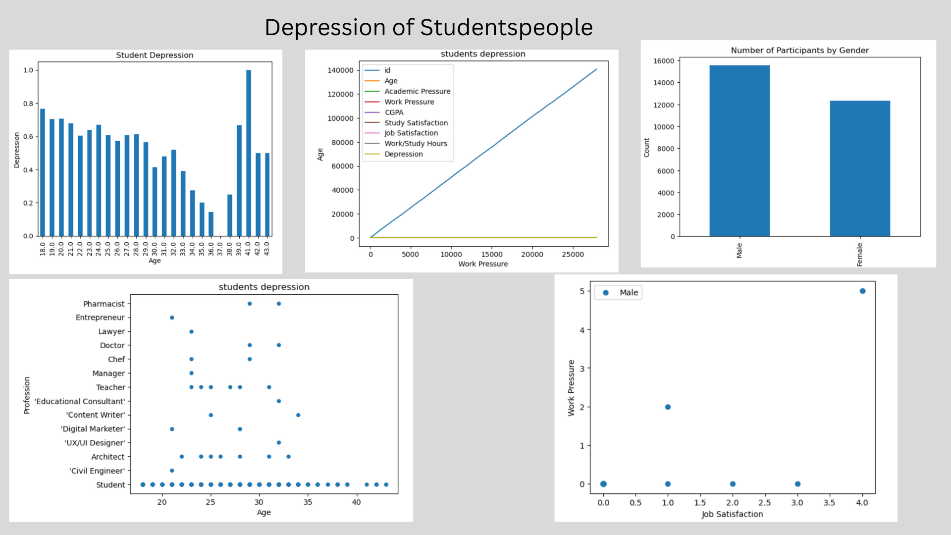
data["Gender"].value_counts()

Gender
Male      15547
Female    12354
Name: count, dtype: int64

data.tail()

data.plot(kind = "line", title = "students depression", xlabel = "Work Pressure", ylabel = "Age")
data

data.plot(kind = "scatter", title = "students depression", x = "Age", y = "Profession")
data

import pandas as pd
import matplotlib.pyplot as plt
grouped = data.groupby("Age")["Depression"].mean()
grouped.plot(kind = "bar")
plt.xlabel("Age")
plt.ylabel("Depression")
plt.title("Student Depression")
plt.show()

import numpy as np
import pandas as pd
import matplotlib.pyplot as plt

# ----------------------------------
# LOAD YOUR DATA
# ----------------------------------
data = pd.read_csv("~/work/rinchen-khandu/datasets/student_depression_dataset.csv")

# Select columns
x_col = "Age"
y_col = "Depression"

# Drop missing values
df = data[[x_col, y_col]].dropna()

x = df[x_col].values
y = df[y_col].values

np.set_printoptions(precision=3)

# ----------------------------------
# POLYNOMIAL FITTING
# ----------------------------------

# First-order (linear) fit
coeff1 = np.polyfit(x, y, 1)
pfit1 = np.poly1d(coeff1)

# Second-order (quadratic) fit
coeff2 = np.polyfit(x, y, 2)
pfit2 = np.poly1d(coeff2)

print(f"First-order fit coefficients (linear): {coeff1}")
print(f"Second-order fit coefficients (quadratic): {coeff2}")

# ----------------------------------
# CREATE SMOOTH FIT CURVES
# ----------------------------------
xmin, xmax = x.min(), x.max()
xfit = np.linspace(xmin, xmax, 200)

yfit1 = pfit1(xfit)
yfit2 = pfit2(xfit)

# ----------------------------------
# PLOTTING
# ----------------------------------
plt.figure(figsize=(8, 6))
plt.plot(x, y, 'o', alpha=0.6, label="Observed data")
plt.plot(xfit, yfit1, 'g-', linewidth=2, label="Linear fit")
plt.plot(xfit, yfit2, 'r-', linewidth=2, label="Quadratic fit")

plt.xlabel(x_col)
plt.ylabel(y_col)
plt.title("Linear vs Quadratic Fit using Real Data")
plt.legend()
plt.grid(True)
plt.show()

First-order fit coefficients (linear): [-0.023  1.173]
Second-order fit coefficients (quadratic): [-0.001  0.019  0.651]

import numpy as np
import pandas as pd
import matplotlib.pyplot as plt

# ----------------------------------
# LOAD YOUR DATA
# ----------------------------------
data = pd.read_csv("~/work/rinchen-khandu/datasets/student_depression_dataset.csv")

# Choose columns
x_col = "Age"          # independent variable
y_col = "Depression"   # dependent variable

# Drop missing values
df = data[[x_col, y_col]].dropna()

x = df[x_col].values
y = df[y_col].values

# ----------------------------------
# SORT DATA (IMPORTANT FOR SMOOTH PLOTS)
# ----------------------------------
idx = np.argsort(x)
x = x[idx]
y = y[idx]

xmin, xmax = x.min(), x.max()
npts = len(x)

# ----------------------------------
# FIT POLYNOMIALS OF DIFFERENT ORDERS
# ----------------------------------
xplot = np.linspace(xmin - 0.2, xmax + 0.2, 300)

# Order 1 (linear)
coeff1 = np.polyfit(x, y, 1)
yfit1 = np.poly1d(coeff1)(xplot)

# Order 4 (moderate complexity)
coeff4 = np.polyfit(x, y, 4)
yfit4 = np.poly1d(coeff4)(xplot)

# Order 15 (high-degree / overfitting)
coeff15 = np.polyfit(x, y, 15)
yfit15 = np.poly1d(coeff15)(xplot)

# ----------------------------------
# PLOTTING
# ----------------------------------
fig = plt.figure(figsize=(8, 6))
fig.canvas.header_visible = False

plt.plot(x, y, 'bo', alpha=0.6, label='Observed data')
plt.plot(xplot, yfit1, 'g-', linewidth=2, label='Order 1 (Underfit)')
plt.plot(xplot, yfit4, 'c-', linewidth=2, label='Order 4')
plt.plot(xplot, yfit15, 'r-', linewidth=2, label='Order 15 (Overfit)')

plt.xlabel(x_col)
plt.ylabel(y_col)
plt.title("Polynomial Fit Comparison Using Real Data")
plt.legend()
plt.grid(True)
plt.show()

/tmp/ipykernel_26369/1382633408.py:44: RankWarning: Polyfit may be poorly conditioned
  coeff15 = np.polyfit(x, y, 15)

import numpy as np
import matplotlib.pyplot as plt
import pandas as pd

#
# load your own data
#
data = pd.read_csv("~/work/rinchen-khandu/datasets/student_depression_dataset.csv")

# ✅ choose the column to analyze
x = data["Age"].dropna().values   # change to "Age" if needed

npts = len(x)

#
# estimate Gaussian parameters from your data
#
mean = np.mean(x)
stddev = np.std(x)

#
# plot histogram and data points
#
plt.hist(x, bins=npts // 50, density=True, alpha=0.6)
plt.plot(x, np.zeros_like(x), '|', ms=10)

#
# plot fitted Gaussian curve
#
xi = np.linspace(mean - 3 * stddev, mean + 3 * stddev, 200)
yi = np.exp(-(xi - mean) ** 2 / (2 * stddev ** 2)) / np.sqrt(2 * np.pi * stddev ** 2)

plt.plot(xi, yi, 'r', linewidth=2)

plt.xlabel("Depression Score")
plt.ylabel("Probability Density")
plt.title("Gaussian Fit to Student Depression Data")
plt.show()

import matplotlib.pyplot as plt
from scipy.spatial import Voronoi, voronoi_plot_2d
import numpy as np
import pandas as pd

#
# k-means parameters
#
nsteps = 1000
momentum = 0.   # (kept for consistency, not used)

#
# import data from CSV
#
data = pd.read_csv('~/work/rinchen-khandu/datasets/student_depression_dataset.csv')

# ✅ FIX: Use Age and Depression columns
# Drop missing values to avoid errors
data = data[["Age", "Depression"]].dropna()

x = data["Age"].values
y = data["Depression"].values

#
# k-means function
#
def kmeans(x, y, momentum, nclusters):

    # choose random initial cluster centers
    indices = np.random.randint(0, len(x), nclusters)
    mux = x[indices]
    muy = y[indices]

    for _ in range(nsteps):

        # distance of each point to each cluster center
        X = np.outer(x, np.ones(len(mux)))
        Y = np.outer(y, np.ones(len(muy)))
        Mux = np.outer(np.ones(len(x)), mux)
        Muy = np.outer(np.ones(len(x)), muy)

        distances = np.sqrt((X - Mux)**2 + (Y - Muy)**2)
        mins = np.argmin(distances, axis=1)

        # update cluster centers
        for i in range(len(mux)):
            index = np.where(mins == i)[0]
            if len(index) > 0:
                mux[i] = np.mean(x[index])
                muy[i] = np.mean(y[index])

    # compute total distance (for elbow method)
    total_distance = 0
    for i in range(len(mux)):
        index = np.where(mins == i)[0]
        total_distance += np.sum(
            np.sqrt((x[index] - mux[i])**2 + (y[index] - muy[i])**2)
        )

    return mux, muy, total_distance


#
# plot k-means clusters
#
def plot_kmeans(x, y, mux, muy):
    plt.figure()
    plt.plot(x, y, '.', alpha=0.6)
    plt.plot(mux, muy, 'r.', markersize=20)
    plt.xlabel("Age")
    plt.ylabel("Depression Score")
    plt.title(f"{len(mux)} clusters (K-Means)")
    plt.show()


#
# plot Voronoi diagram
#
def plot_Voronoi(x, y, mux, muy):
    plt.figure()
    plt.plot(x, y, '.', alpha=0.6)

    vor = Voronoi(np.column_stack((mux, muy)))
    voronoi_plot_2d(
        vor,
        show_points=True,
        show_vertices=False,
        point_size=20
    )

    plt.xlabel("Age")
    plt.ylabel("Sleep Duration")
    plt.title(f"{len(mux)} clusters (Voronoi)")
    plt.show()


#
# run clustering for different cluster counts
#
distances = np.zeros(5)

mux, muy, distances[0] = kmeans(x, y, momentum, 1)
plot_kmeans(x, y, mux, muy)

mux, muy, distances[1] = kmeans(x, y, momentum, 2)
plot_kmeans(x, y, mux, muy)

mux, muy, distances[2] = kmeans(x, y, momentum, 3)
plot_Voronoi(x, y, mux, muy)

mux, muy, distances[3] = kmeans(x, y, momentum, 4)
plot_Voronoi(x, y, mux, muy)

mux, muy, distances[4] = kmeans(x, y, momentum, 5)
plot_Voronoi(x, y, mux, muy)


#
# elbow method plot
#
plt.figure()
plt.plot(np.arange(1, 6), distances, 'o-')
plt.xlabel("Number of clusters")
plt.ylabel("Total distance to clusters")
plt.title("Elbow Method (Age vs Depression)")
plt.show()

---------------------------------------------------------------------------
QhullError                                Traceback (most recent call last)
Cell In[18], line 109
    106 plot_kmeans(x, y, mux, muy)
    108 mux, muy, distances[2] = kmeans(x, y, momentum, 3)
--> 109 plot_Voronoi(x, y, mux, muy)
    111 mux, muy, distances[3] = kmeans(x, y, momentum, 4)
    112 plot_Voronoi(x, y, mux, muy)

Cell In[18], line 83, in plot_Voronoi(x, y, mux, muy)
     80 plt.figure()
     81 plt.plot(x, y, '.', alpha=0.6)
---> 83 vor = Voronoi(np.column_stack((mux, muy)))
     84 voronoi_plot_2d(
     85     vor,
     86     show_points=True,
     87     show_vertices=False,
     88     point_size=20
     89 )
     91 plt.xlabel("Age")

File scipy/spatial/_qhull.pyx:2680, in scipy.spatial._qhull.Voronoi.__init__()

File scipy/spatial/_qhull.pyx:356, in scipy.spatial._qhull._Qhull.__init__()

QhullError: QH6154 Qhull precision error: Initial simplex is flat (facet 1 is coplanar with the interior point)

While executing:  | qhull v Qc Qz Qbb
Options selected for Qhull 2020.2.r 2020/08/31:
  run-id 1695218816  voronoi  Qcoplanar-keep  Qz-infinity-point  Qbbound-last
  _pre-merge  _zero-centrum  Qinterior-keep  Pgood  _max-width 11
  Error-roundoff 4.3e-14  _one-merge 3e-13  Visible-distance 8.6e-14
  U-max-coplanar 8.6e-14  Width-outside 1.7e-13  _wide-facet 5.1e-13
  _maxoutside 3.4e-13

The input to qhull appears to be less than 3 dimensional, or a
computation has overflowed.

Qhull could not construct a clearly convex simplex from points:
- p3(v4):    25     0    31
- p0(v3):    25     0    10
- p2(v2):    31     0    26
- p1(v1):    20     0     0

The center point is coplanar with a facet, or a vertex is coplanar
with a neighboring facet.  The maximum round off error for
computing distances is 4.3e-14.  The center point, facets and distances
to the center point are as follows:

center point     25.2        0    16.91

facet p0 p2 p1 distance=    0
facet p3 p2 p1 distance=    0
facet p3 p0 p1 distance=    0
facet p3 p0 p2 distance=    0

These points either have a maximum or minimum x-coordinate, or
they maximize the determinant for k coordinates.  Trial points
are first selected from points that maximize a coordinate.

The min and max coordinates for each dimension are:
  0:     19.92     30.87  difference= 10.95
  1:         0         0  difference=    0
  2:         0     30.87  difference= 30.87

If the input should be full dimensional, you have several options that
may determine an initial simplex:
  - use 'QJ'  to joggle the input and make it full dimensional
  - use 'QbB' to scale the points to the unit cube
  - use 'QR0' to randomly rotate the input for different maximum points
  - use 'Qs'  to search all points for the initial simplex
  - use 'En'  to specify a maximum roundoff error less than 4.3e-14.
  - trace execution with 'T3' to see the determinant for each point.

If the input is lower dimensional:
  - use 'QJ' to joggle the input and make it full dimensional
  - use 'Qbk:0Bk:0' to delete coordinate k from the input.  You should
    pick the coordinate with the least range.  The hull will have the
    correct topology.
  - determine the flat containing the points, rotate the points
    into a coordinate plane, and delete the other coordinates.
  - add one or more points to make the input full dimensional.

import matplotlib.pyplot as plt
import numpy as np
import pandas as pd

#
# Load your own data
#
data = pd.read_csv("~/work/rinchen-khandu/datasets/student_depression_dataset.csv")
data = data[["Age", "Depression"]].dropna()

x = data["Age"].values
y = data["Depression"].values

# sort data (important for plotting smooth curves)
idx = np.argsort(x)
x = x[idx]
y = y[idx]

npts = len(x)

#
# function cluster-weighted modeling parameters
#
nclusters = 5
minvar = 0.01
niterations = 100
np.random.seed(10)

xplot = np.copy(x)
nplot = npts

#
# initialize parameters
#
mux = np.random.choice(x, nclusters)
beta = 0.1 * np.random.rand(3, nclusters)
varx = np.ones(nclusters)
vary = np.ones(nclusters)
pc = np.ones(nclusters) / nclusters

#
# ---------- BEFORE ITERATION ----------
#
pxgc = np.exp(-(np.outer(x, np.ones(nclusters))
               - np.outer(np.ones(npts), mux))**2
              / (2 * np.outer(np.ones(npts), varx))) \
       / np.sqrt(2 * np.pi * np.outer(np.ones(npts), varx))

pygxc = np.exp(-(np.outer(y, np.ones(nclusters))
                - (np.outer(np.ones(npts), beta[0, :])
                   + np.outer(x, beta[1, :])
                   + np.outer(x * x, beta[2, :])))**2
               / (2 * np.outer(np.ones(npts), vary))) \
        / np.sqrt(2 * np.pi * np.outer(np.ones(npts), vary))

pxc = pxgc * np.outer(np.ones(npts), pc)
pxyc = pygxc * pxc
pcgxy = pxyc / np.outer(np.sum(pxyc, 1), np.ones(nclusters))

plt.figure()
plt.plot(x, y, '.', alpha=0.6)

yplot = np.sum((np.outer(np.ones(nplot), beta[0, :])
               + np.outer(x, beta[1, :])
               + np.outer(x * x, beta[2, :])) * pxc, 1) / np.sum(pxc, 1)
plt.plot(xplot, yplot)

yvarplot = np.sum((vary +
                  (np.outer(np.ones(nplot), beta[0, :])
                   + np.outer(x, beta[1, :])
                   + np.outer(x * x, beta[2, :]))**2) * pxc, 1) \
           / np.sum(pxc, 1) - yplot**2

ystdplot = np.sqrt(yvarplot)
plt.plot(xplot, yplot + ystdplot, 'k--')
plt.plot(xplot, yplot - ystdplot, 'k--')

plt.title("Function Clusters BEFORE EM Iteration")
plt.xlabel("Age")
plt.ylabel("Depression Score")
plt.show()

#
# ---------- EM ITERATION ----------
#
for step in range(niterations):

    pxgc = np.exp(-(np.outer(x, np.ones(nclusters))
                   - np.outer(np.ones(npts), mux))**2
                  / (2 * np.outer(np.ones(npts), varx))) \
           / np.sqrt(2 * np.pi * np.outer(np.ones(npts), varx))

    pygxc = np.exp(-(np.outer(y, np.ones(nclusters))
                    - (np.outer(np.ones(npts), beta[0, :])
                       + np.outer(x, beta[1, :])
                       + np.outer(x * x, beta[2, :])))**2
                   / (2 * np.outer(np.ones(npts), vary))) \
            / np.sqrt(2 * np.pi * np.outer(np.ones(npts), vary))

    pxc = pxgc * np.outer(np.ones(npts), pc)
    pxyc = pygxc * pxc
    pcgxy = pxyc / np.outer(np.sum(pxyc, 1), np.ones(nclusters))

    pc = np.sum(pcgxy, 0) / npts
    mux = np.sum(np.outer(x, np.ones(nclusters)) * pcgxy, 0) / (npts * pc)
    varx = minvar + np.sum((np.outer(x, np.ones(nclusters))
                            - np.outer(np.ones(npts), mux))**2
                           * pcgxy, 0) / (npts * pc)

    a = np.array([
        np.sum(np.outer(y, np.ones(nclusters)) * pcgxy, 0) / (npts * pc),
        np.sum(np.outer(y * x, np.ones(nclusters)) * pcgxy, 0) / (npts * pc),
        np.sum(np.outer(y * x * x, np.ones(nclusters)) * pcgxy, 0) / (npts * pc)
    ])

    B = np.zeros((3, 3, nclusters))
    for c in range(nclusters):
        B[:, :, c] = [
            [1,
             np.sum(x * pcgxy[:, c]) / (npts * pc[c]),
             np.sum(x * x * pcgxy[:, c]) / (npts * pc[c])],
            [np.sum(x * pcgxy[:, c]) / (npts * pc[c]),
             np.sum(x * x * pcgxy[:, c]) / (npts * pc[c]),
             np.sum(x * x * x * pcgxy[:, c]) / (npts * pc[c])],
            [np.sum(x * x * pcgxy[:, c]) / (npts * pc[c]),
             np.sum(x * x * x * pcgxy[:, c]) / (npts * pc[c]),
             np.sum(x * x * x * x * pcgxy[:, c]) / (npts * pc[c])]
        ]
        beta[:, c] = np.linalg.inv(B[:, :, c]) @ a[:, c]

    vary = minvar + np.sum((np.outer(y, np.ones(nclusters))
                            - (np.outer(np.ones(npts), beta[0, :])
                               + np.outer(x, beta[1, :])
                               + np.outer(x * x, beta[2, :])))**2
                           * pcgxy, 0) / (npts * pc)

#
# ---------- AFTER ITERATION ----------
#
plt.figure()
plt.plot(x, y, '.', alpha=0.6)

yplot = np.sum((np.outer(np.ones(nplot), beta[0, :])
               + np.outer(x, beta[1, :])
               + np.outer(x * x, beta[2, :])) * pxc, 1) / np.sum(pxc, 1)
plt.plot(xplot, yplot)

ystdplot = np.sqrt(yvarplot)
plt.plot(xplot, yplot + ystdplot, 'k--')
plt.plot(xplot, yplot - ystdplot, 'k--')

plt.title("Function Clusters AFTER EM Iteration")
plt.xlabel("Age")
plt.ylabel("Depression Score")
plt.show()

/tmp/ipykernel_26369/3832536625.py:58: RuntimeWarning: invalid value encountered in divide
  pcgxy = pxyc / np.outer(np.sum(pxyc, 1), np.ones(nclusters))

/tmp/ipykernel_26369/3832536625.py:102: RuntimeWarning: invalid value encountered in divide
  pcgxy = pxyc / np.outer(np.sum(pxyc, 1), np.ones(nclusters))

import numpy as np
import pandas as pd
import matplotlib.pyplot as plt
from sklearn.decomposition import PCA
np.set_printoptions(precision=2)

#
# load your own data
#
data = pd.read_csv("~/work/rinchen-khandu/datasets/student_depression_dataset.csv")

# select numerical columns only
numerical_cols = data.select_dtypes(include=[np.number]).columns
X = data[numerical_cols].dropna().values

print(f"Data shape (records, features): {X.shape}")

#
# optional: plot vs first two columns
#
plt.scatter(X[:, 0], X[:, 1], c='blue', alpha=0.6)
plt.xlabel(numerical_cols[0])
plt.ylabel(numerical_cols[1])
plt.title(f"{numerical_cols[0]} vs {numerical_cols[1]}")
plt.show()

#
# standardize data (zero mean, unit variance)
#
X_mean = np.mean(X, axis=0)
X_std = np.std(X, axis=0)
Xscale = (X - X_mean) / np.where(X_std > 0, X_std, 1)

print(f"Standardized data mean: {np.mean(Xscale):.2f}, variance: {np.var(Xscale):.2f}")

#
# do PCA
#
n_components = min(50, Xshape := Xscale.shape[1])  # max 50 or # of features
pca = PCA(n_components=n_components)
pca.fit(Xscale)
Xpca = pca.transform(Xscale)

#
# plot explained variance
#
plt.plot(pca.explained_variance_, 'o-')
plt.xlabel('PCA component')
plt.ylabel('Explained variance')
plt.title('PCA Explained Variance')
plt.show()

#
# plot first two PCA components
#
plt.scatter(Xpca[:, 0], Xpca[:, 1], c='green', s=20, alpha=0.6)
plt.xlabel("Principal component 1")
plt.ylabel("Principal component 2")
plt.title("Data projected on first two PCA components")
plt.show()

Data shape (records, features): (27901, 9)

Standardized data mean: 0.00, variance: 1.00

	id	Gender	Age	City	Profession	Academic Pressure	Work Pressure	CGPA	Study Satisfaction	Job Satisfaction	Sleep Duration	Dietary Habits	Degree	Have you ever had suicidal thoughts ?	Work/Study Hours	Financial Stress	Family History of Mental Illness	Depression
0	2	Male	33.0	Visakhapatnam	Student	5.0	0.0	8.97	2.0	0.0	'5-6 hours'	Healthy	B.Pharm	Yes	3.0	1.0	No	1
1	8	Female	24.0	Bangalore	Student	2.0	0.0	5.90	5.0	0.0	'5-6 hours'	Moderate	BSc	No	3.0	2.0	Yes	0
2	26	Male	31.0	Srinagar	Student	3.0	0.0	7.03	5.0	0.0	'Less than 5 hours'	Healthy	BA	No	9.0	1.0	Yes	0
3	30	Female	28.0	Varanasi	Student	3.0	0.0	5.59	2.0	0.0	'7-8 hours'	Moderate	BCA	Yes	4.0	5.0	Yes	1
4	32	Female	25.0	Jaipur	Student	4.0	0.0	8.13	3.0	0.0	'5-6 hours'	Moderate	M.Tech	Yes	1.0	1.0	No	0
...	...	...	...	...	...	...	...	...	...	...	...	...	...	...	...	...	...	...
27896	140685	Female	27.0	Surat	Student	5.0	0.0	5.75	5.0	0.0	'5-6 hours'	Unhealthy	'Class 12'	Yes	7.0	1.0	Yes	0
27897	140686	Male	27.0	Ludhiana	Student	2.0	0.0	9.40	3.0	0.0	'Less than 5 hours'	Healthy	MSc	No	0.0	3.0	Yes	0
27898	140689	Male	31.0	Faridabad	Student	3.0	0.0	6.61	4.0	0.0	'5-6 hours'	Unhealthy	MD	No	12.0	2.0	No	0
27899	140690	Female	18.0	Ludhiana	Student	5.0	0.0	6.88	2.0	0.0	'Less than 5 hours'	Healthy	'Class 12'	Yes	10.0	5.0	No	1
27900	140699	Male	27.0	Patna	Student	4.0	0.0	9.24	1.0	0.0	'Less than 5 hours'	Healthy	BCA	Yes	2.0	3.0	Yes	1

	id	Gender	Age	City	Profession	Academic Pressure	CGPA	Study Satisfaction	Sleep Duration	Dietary Habits	Degree	Have you ever had suicidal thoughts ?	Work/Study Hours	Financial Stress	Family History of Mental Illness	Depression
0	2	Male	33.0	Visakhapatnam	Student	5.0	8.97	2.0	'5-6 hours'	Healthy	B.Pharm	Yes	3.0	1.0	No	1
1	8	Female	24.0	Bangalore	Student	2.0	5.90	5.0	'5-6 hours'	Moderate	BSc	No	3.0	2.0	Yes	0
2	26	Male	31.0	Srinagar	Student	3.0	7.03	5.0	'Less than 5 hours'	Healthy	BA	No	9.0	1.0	Yes	0
3	30	Female	28.0	Varanasi	Student	3.0	5.59	2.0	'7-8 hours'	Moderate	BCA	Yes	4.0	5.0	Yes	1
4	32	Female	25.0	Jaipur	Student	4.0	8.13	3.0	'5-6 hours'	Moderate	M.Tech	Yes	1.0	1.0	No	0

	id	Age	Academic Pressure	Work Pressure	CGPA	Study Satisfaction	Job Satisfaction	Work/Study Hours	Depression
count	27901.000000	27901.000000	27901.000000	27901.000000	27901.000000	27901.000000	27901.000000	27901.000000	27901.000000
mean	70442.149421	25.822300	3.141214	0.000430	7.656104	2.943837	0.000681	7.156984	0.585499
std	40641.175216	4.905687	1.381465	0.043992	1.470707	1.361148	0.044394	3.707642	0.492645
min	2.000000	18.000000	0.000000	0.000000	0.000000	0.000000	0.000000	0.000000	0.000000
25%	35039.000000	21.000000	2.000000	0.000000	6.290000	2.000000	0.000000	4.000000	0.000000
50%	70684.000000	25.000000	3.000000	0.000000	7.770000	3.000000	0.000000	8.000000	1.000000
75%	105818.000000	30.000000	4.000000	0.000000	8.920000	4.000000	0.000000	10.000000	1.000000
max	140699.000000	59.000000	5.000000	5.000000	10.000000	5.000000	4.000000	12.000000	1.000000

	id	Gender	Age	City	Profession	Academic Pressure	CGPA	Study Satisfaction	Sleep Duration	Dietary Habits	Degree	Have you ever had suicidal thoughts ?	Work/Study Hours	Financial Stress	Family History of Mental Illness	Depression
27896	140685	Female	27.0	Surat	Student	5.0	5.75	5.0	'5-6 hours'	Unhealthy	'Class 12'	Yes	7.0	1.0	Yes	0
27897	140686	Male	27.0	Ludhiana	Student	2.0	9.40	3.0	'Less than 5 hours'	Healthy	MSc	No	0.0	3.0	Yes	0
27898	140689	Male	31.0	Faridabad	Student	3.0	6.61	4.0	'5-6 hours'	Unhealthy	MD	No	12.0	2.0	No	0
27899	140690	Female	18.0	Ludhiana	Student	5.0	6.88	2.0	'Less than 5 hours'	Healthy	'Class 12'	Yes	10.0	5.0	No	1
27900	140699	Male	27.0	Patna	Student	4.0	9.24	1.0	'Less than 5 hours'	Healthy	BCA	Yes	2.0	3.0	Yes	1

	id	Gender	Age	City	Profession	Academic Pressure	Work Pressure	CGPA	Study Satisfaction	Job Satisfaction	Sleep Duration	Dietary Habits	Degree	Have you ever had suicidal thoughts ?	Work/Study Hours	Financial Stress	Family History of Mental Illness	Depression
0	2	Male	33.0	Visakhapatnam	Student	5.0	0.0	8.97	2.0	0.0	'5-6 hours'	Healthy	B.Pharm	Yes	3.0	1.0	No	1
1	8	Female	24.0	Bangalore	Student	2.0	0.0	5.90	5.0	0.0	'5-6 hours'	Moderate	BSc	No	3.0	2.0	Yes	0
2	26	Male	31.0	Srinagar	Student	3.0	0.0	7.03	5.0	0.0	'Less than 5 hours'	Healthy	BA	No	9.0	1.0	Yes	0
3	30	Female	28.0	Varanasi	Student	3.0	0.0	5.59	2.0	0.0	'7-8 hours'	Moderate	BCA	Yes	4.0	5.0	Yes	1
4	32	Female	25.0	Jaipur	Student	4.0	0.0	8.13	3.0	0.0	'5-6 hours'	Moderate	M.Tech	Yes	1.0	1.0	No	0
...	...	...	...	...	...	...	...	...	...	...	...	...	...	...	...	...	...	...
27896	140685	Female	27.0	Surat	Student	5.0	0.0	5.75	5.0	0.0	'5-6 hours'	Unhealthy	'Class 12'	Yes	7.0	1.0	Yes	0
27897	140686	Male	27.0	Ludhiana	Student	2.0	0.0	9.40	3.0	0.0	'Less than 5 hours'	Healthy	MSc	No	0.0	3.0	Yes	0
27898	140689	Male	31.0	Faridabad	Student	3.0	0.0	6.61	4.0	0.0	'5-6 hours'	Unhealthy	MD	No	12.0	2.0	No	0
27899	140690	Female	18.0	Ludhiana	Student	5.0	0.0	6.88	2.0	0.0	'Less than 5 hours'	Healthy	'Class 12'	Yes	10.0	5.0	No	1
27900	140699	Male	27.0	Patna	Student	4.0	0.0	9.24	1.0	0.0	'Less than 5 hours'	Healthy	BCA	Yes	2.0	3.0	Yes	1

Presentation¶

Tools¶

Pandas¶

Numpy¶

Matplotlib¶

Scikit learn¶

student_depression_dataset¶

Data Visualization¶

Line Graph¶

Students Depression¶

Scatter plot¶

Functions and Fitting¶

Polyfit and Linear¶

Probability¶

Density and Estimation¶

Voronoi tesselation¶

Modeling Functions¶

Transformation¶

Principal Components Analysis (PCA)¶

References¶