Week 1: Introduction¶

This week we will identify a dataset which we will use to explore and make our self familiar with the tools.

Assignment¶

Work Environment: Setting the work environment
Dataset: Identification and brief description about the dataset
Data Analysis

Work Environment¶

Setting Jupyter Notebooks in VS Code as my work environment for this course.¶

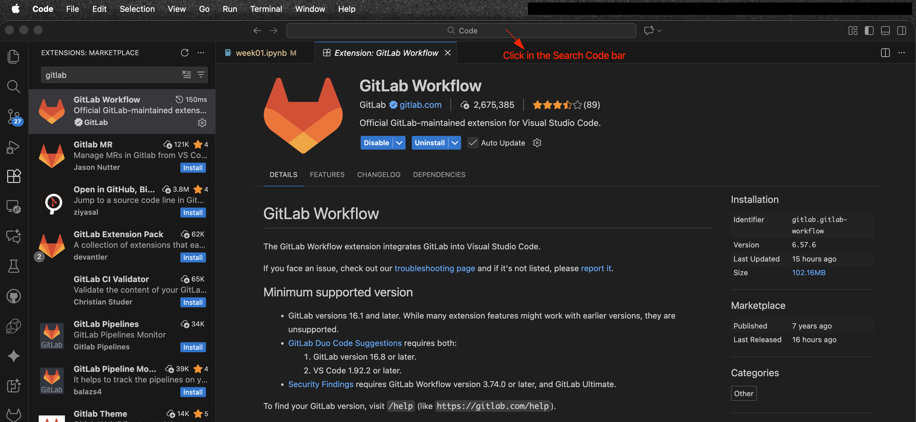
Install GitLab Workflow extension in VS Code.
Generate a Personal Access Token in GitLab.
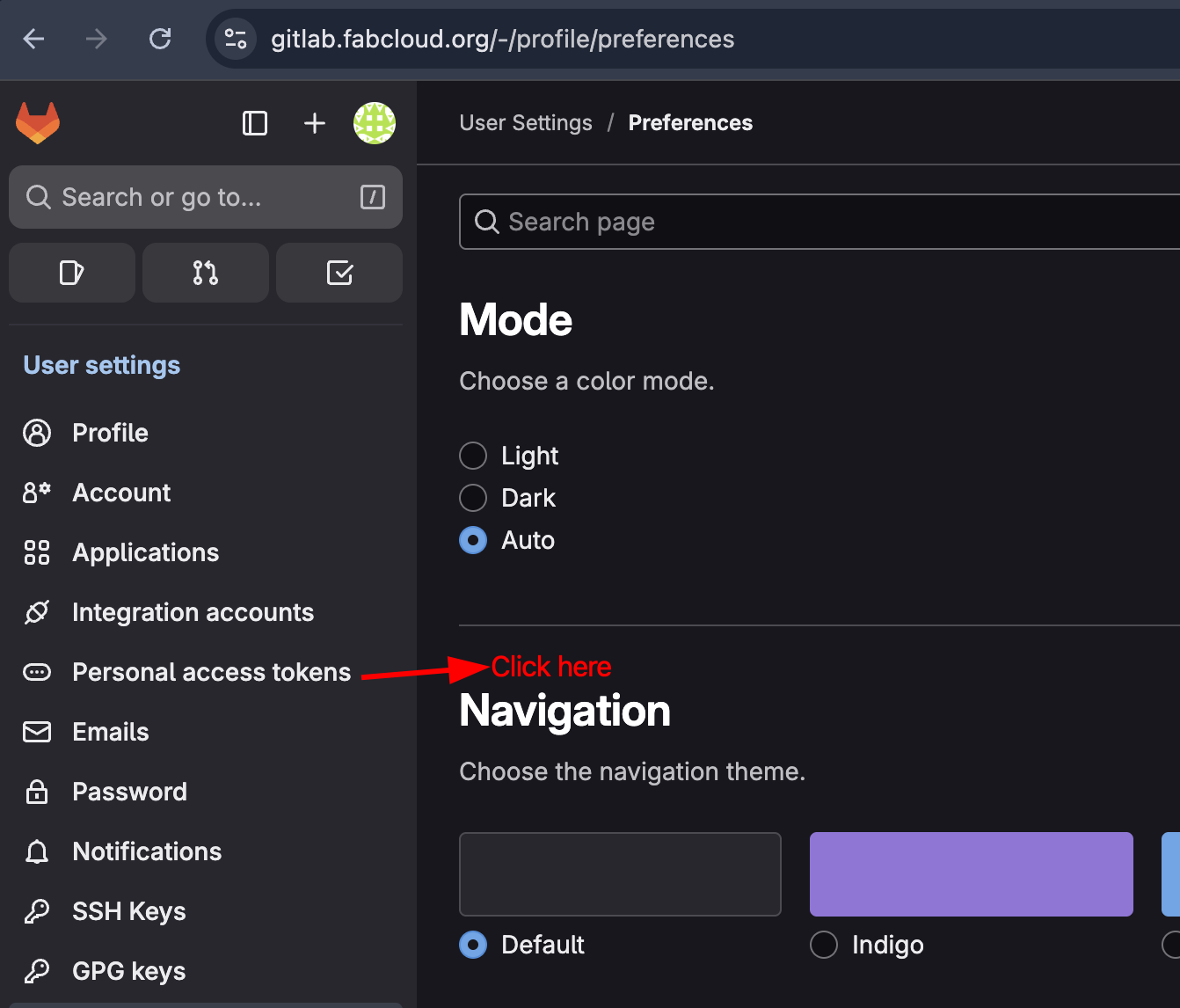
- Go to your GitLab profile settings.
- Click on Preferences > Personal Access Tokens > Add new token.
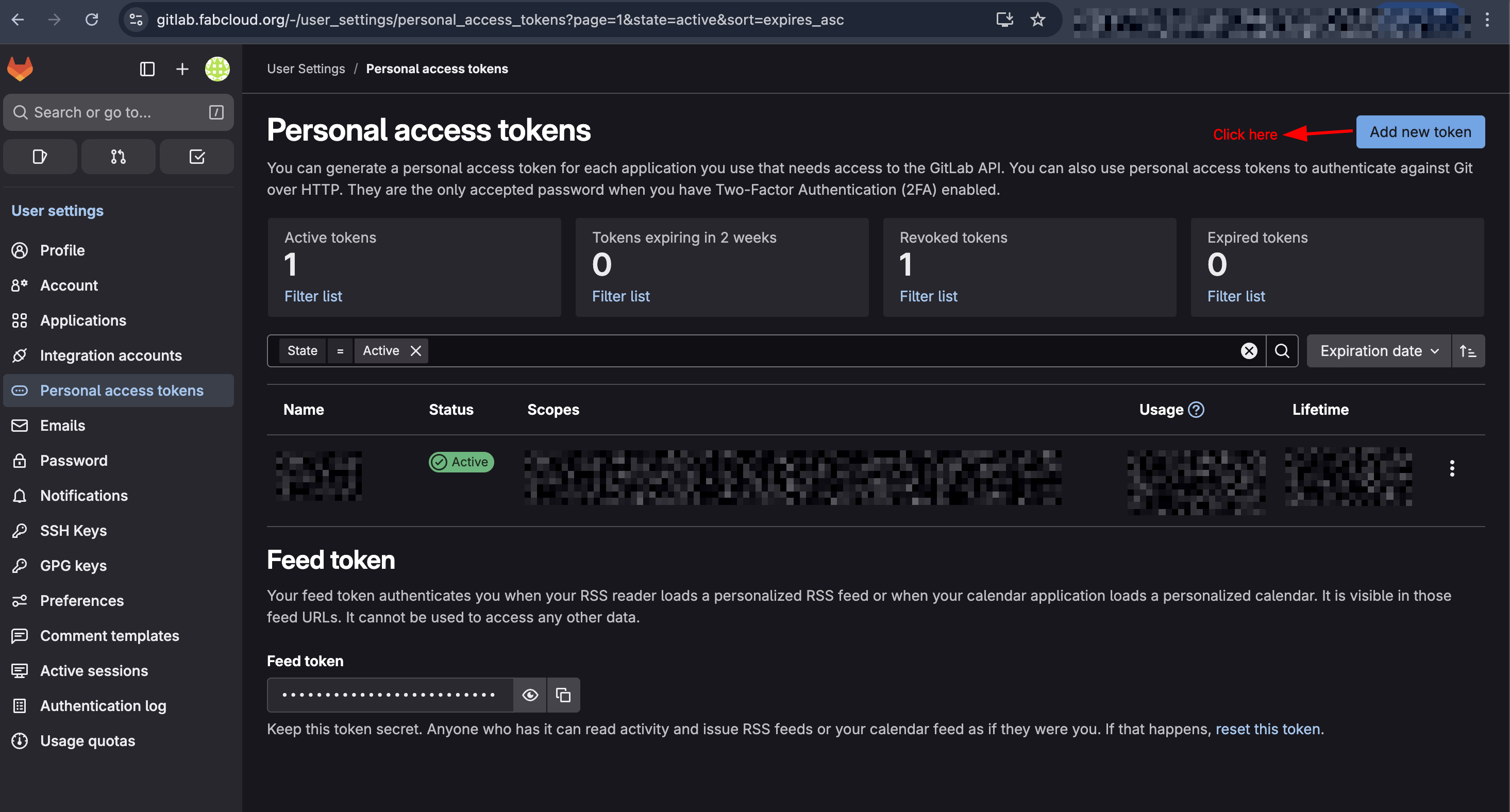
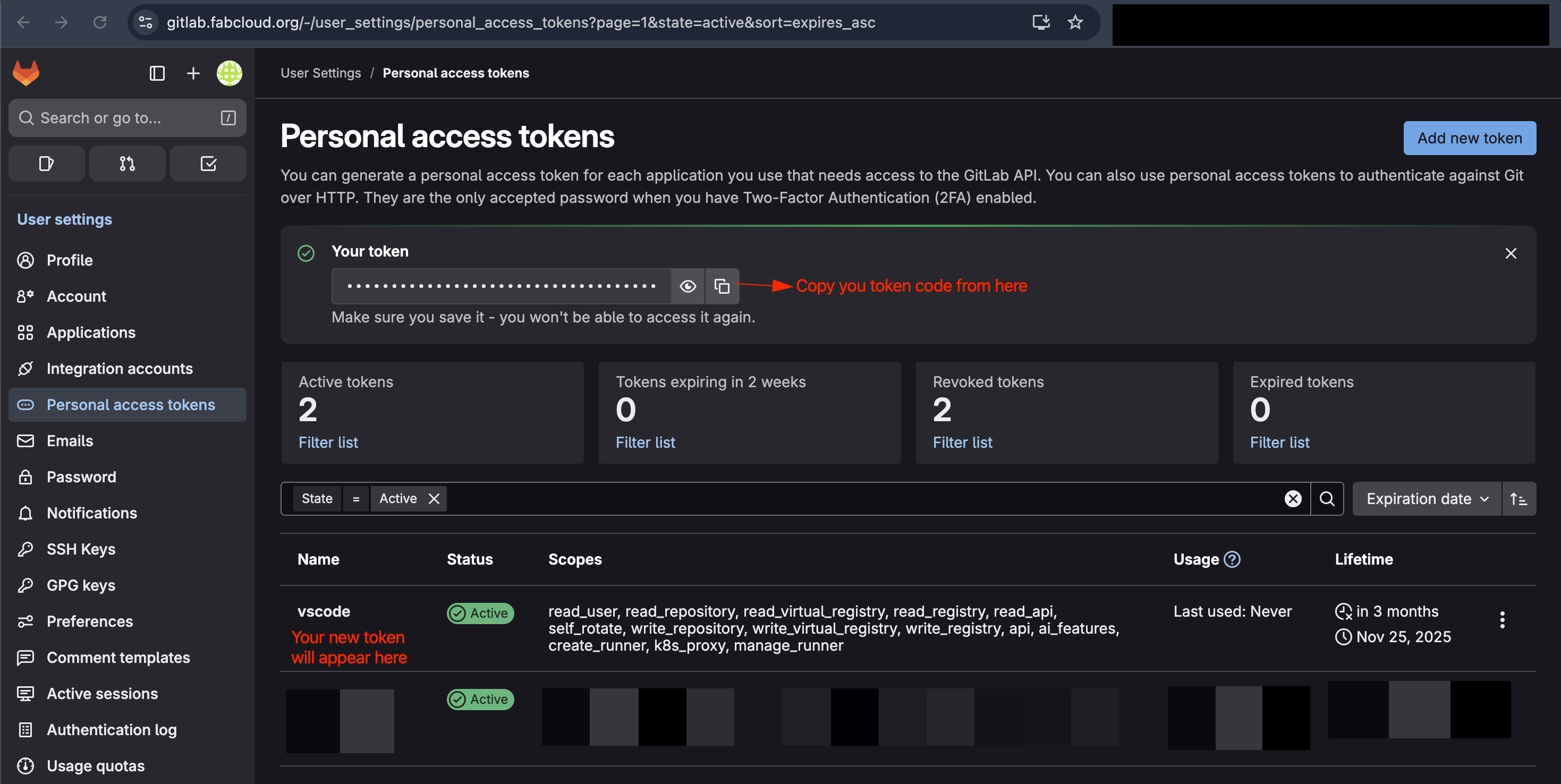
- Now enter token name of your choice, select the expiry date and the required scopes. Finally click on "Create token" button.
- Copy the generated token and save it for later use as you won't be able to see it again.
Now add your GitLab account details in VS Code.
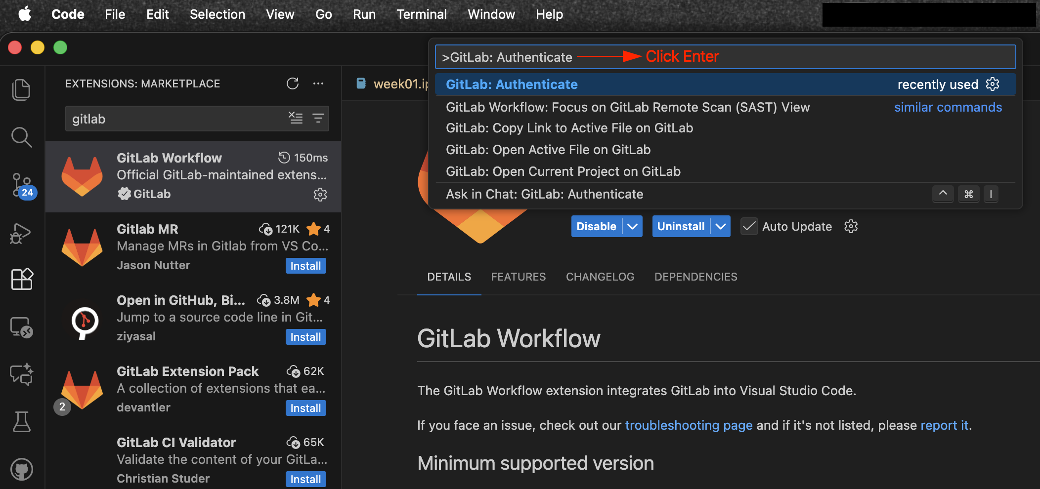
- Open Command Palette (Command+Shift+P on Mac) and search for "GitLab: Authenticate"
  OR
  Click on the Search Code bar at the top and search for ">GitLab: Authenticate" (works for all OS).
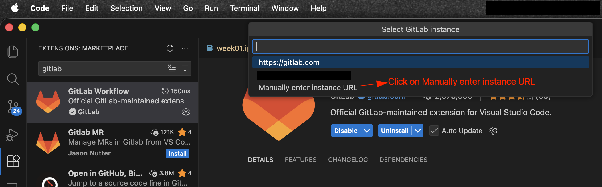
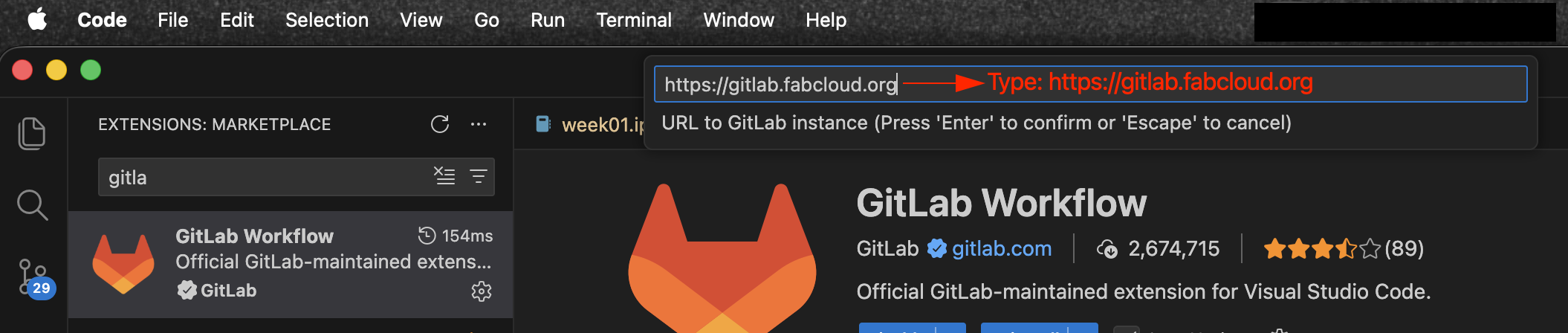
- Now enter your GitLab instance URL (https://gitlab.fabcloud.org) and press Enter.
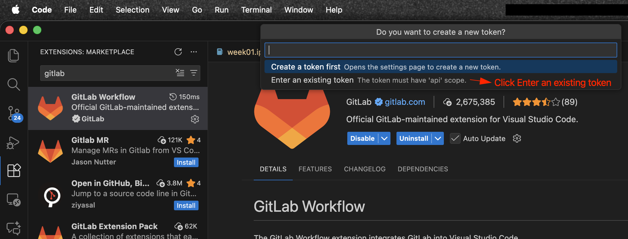
- Now click Enter an existing token and enter the Personal Access Token you generated earlier and press Enter.
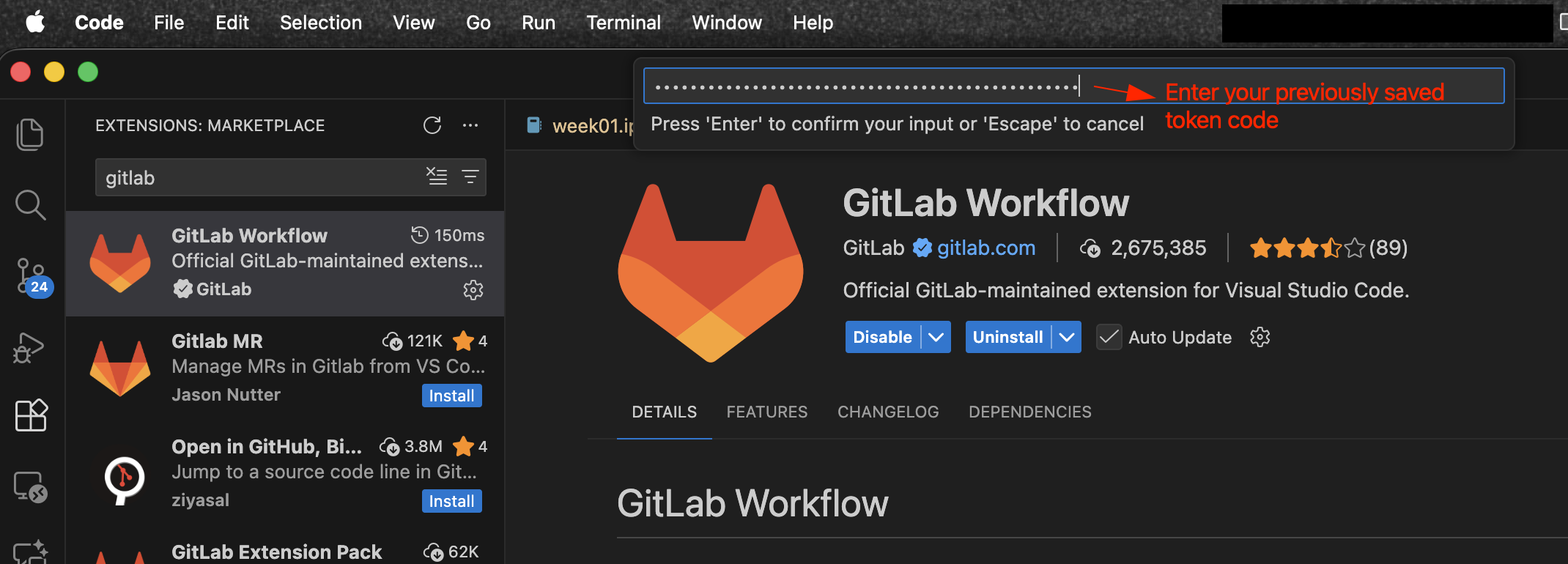
- You will see a notification confirming that you have successfully authenticated your GitLab account in VS.
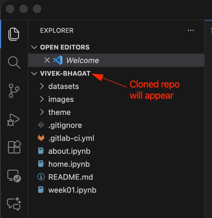
Clone the course repository from GitLab to your local machine.
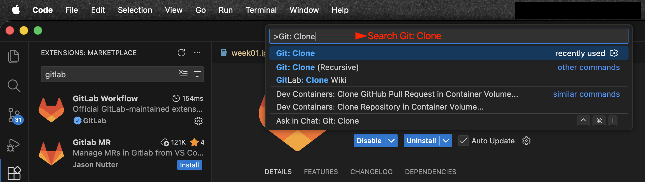
- Open Command Palette (Command+Shift+P on Mac) and search for "Git: Clone"
  OR
  Click on the Search Code bar at the top and search for ">Git: Clone" (works for all OS).
- Now click "Clone from GitLab".
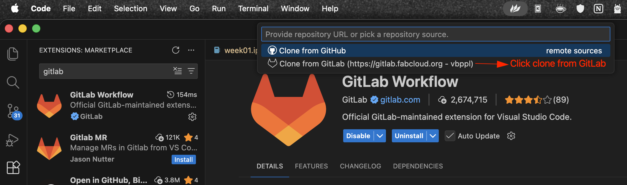
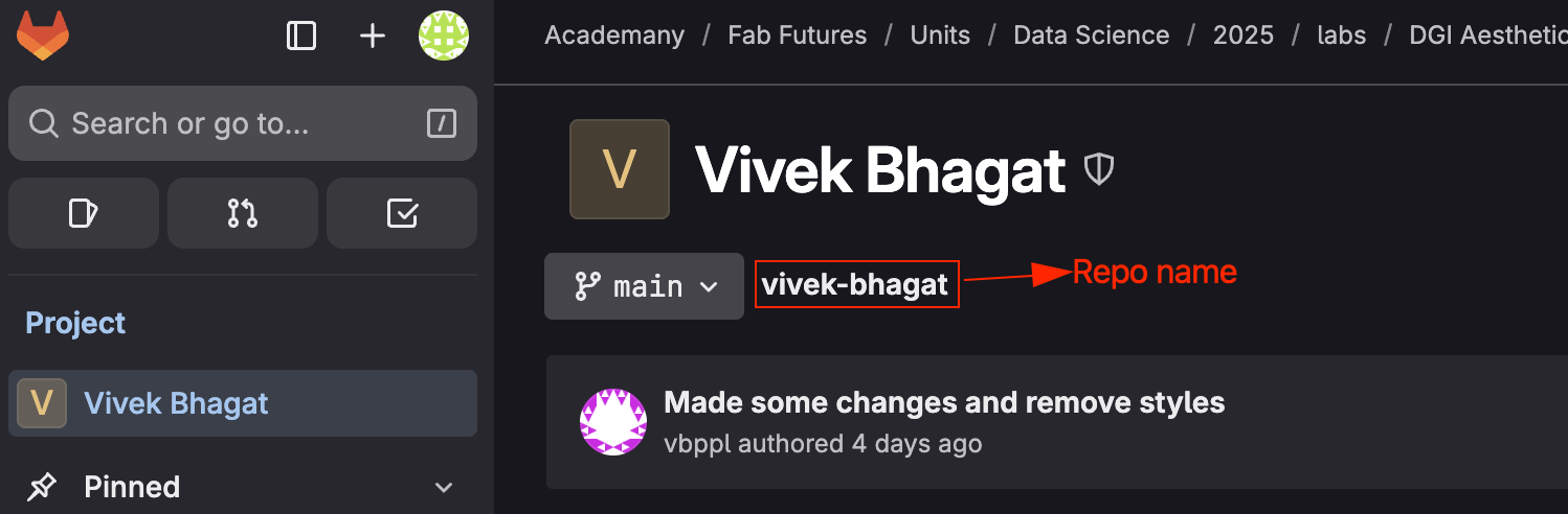
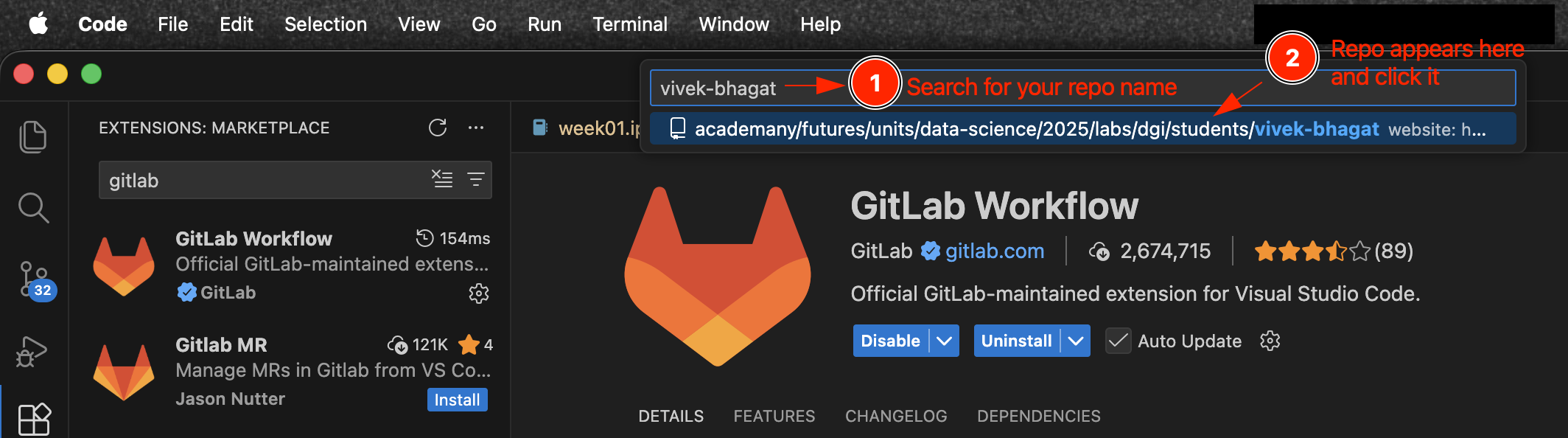
- Search for the repository you want to clone and select it. You can find course repo in gitlab.
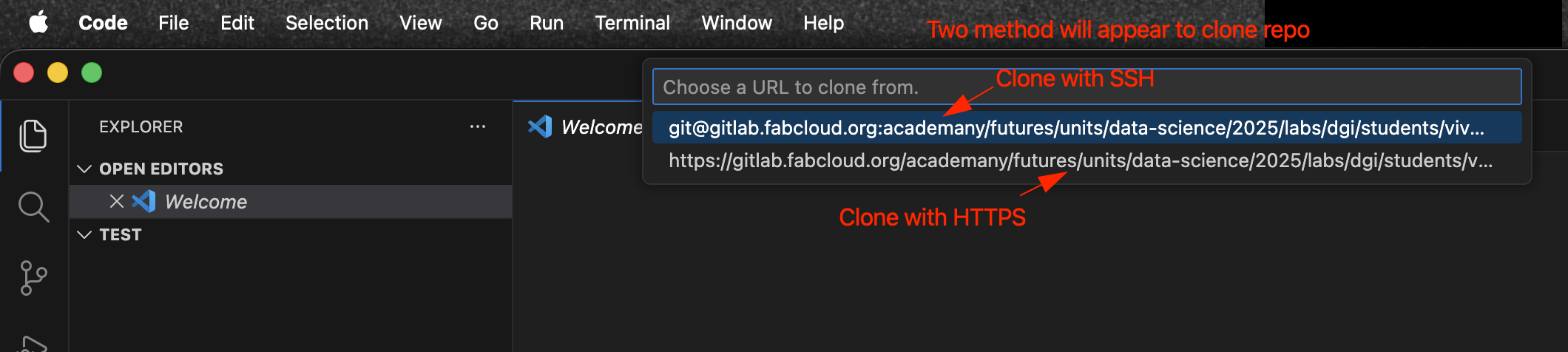
- Now select the cloning method, select "Clone with HTTPS".
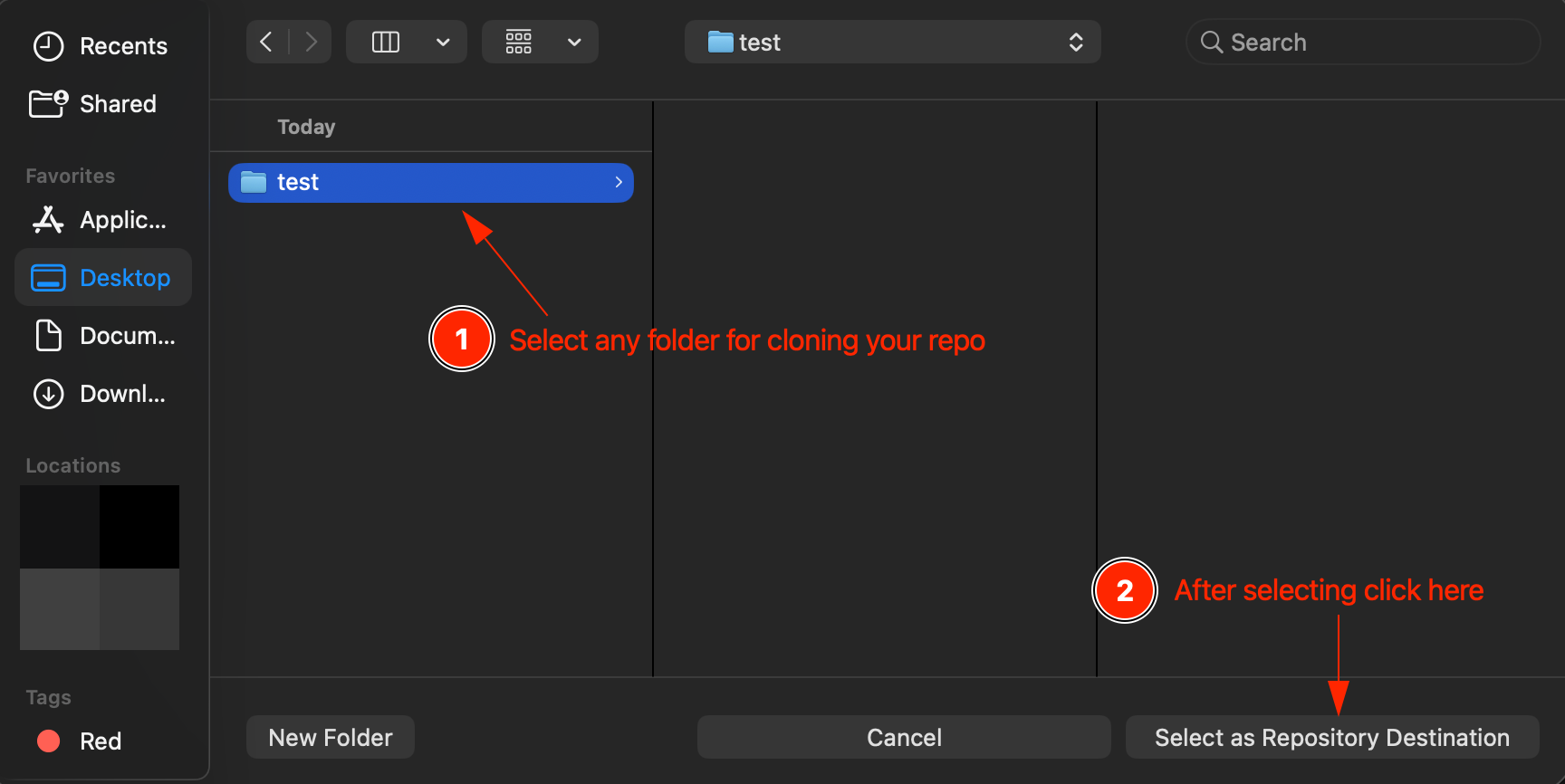
- Now select the local directory where you want to clone the repository and click "Select Repository Location".

Push, Pull, Commit changes to the repository directly from VS Code or from other IDE.
Let’s assume we need to add a image “home” to the repository to modify the homepage.

git add images/home.png  	#Stage the file home.png for commit.  
git commit -m "Added image 'home' for home page"  # Commit message should be relevant to the changes made.  
git push origin main

Let's assume we need to add multiple images starting with "clone_repo_" to the repository. Push Commit

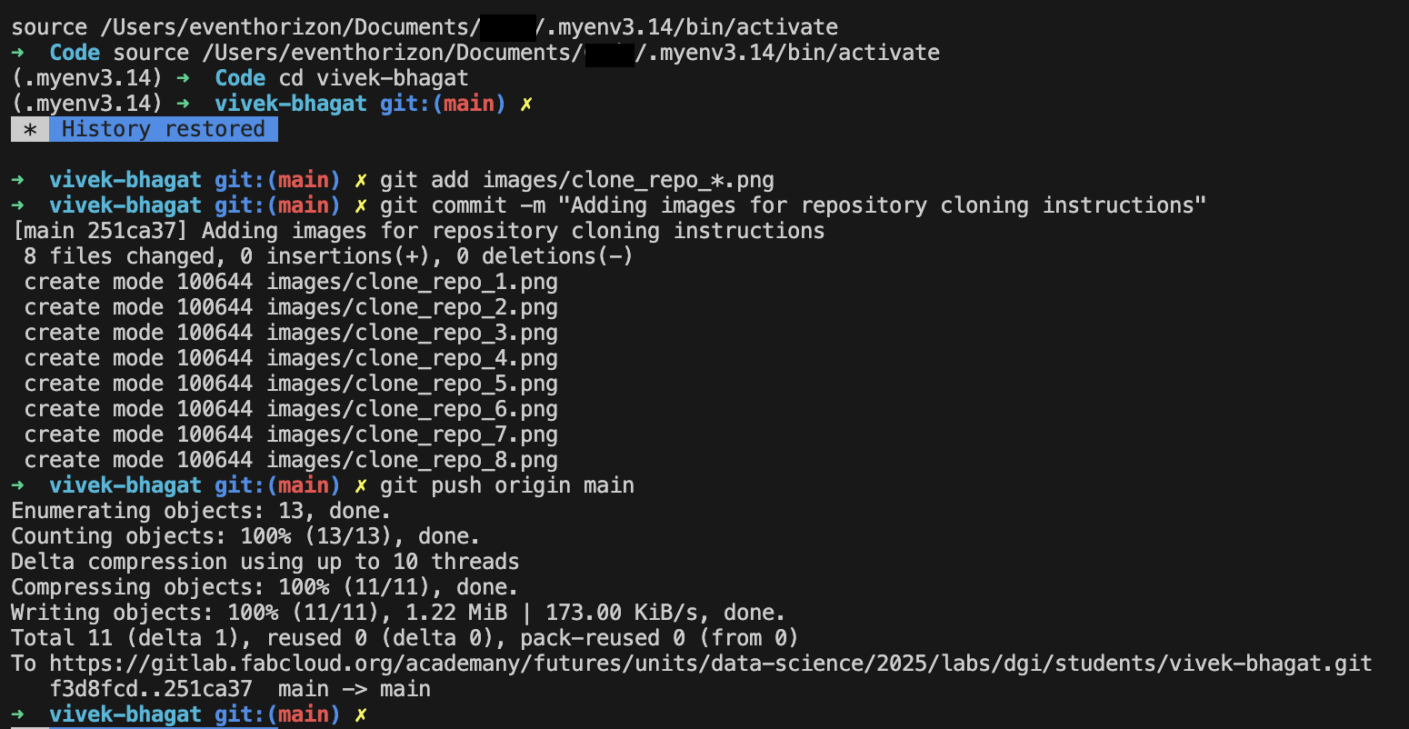
git add images/clone_repo_*.png  	#Stage all the files starting with clone_repo_ for commit.
git commit -m "Adding images for repository cloning instructions"  
git push origin main

Let's assume we staged a file and then realized we don't want to commit it. Push Commit 2

git add images/push_commit.png  	#Stage the file push_commit.png for commit.
git reset HEAD images/push_commit.png  	#Unstage the file ready to commit.

Dataset¶

HIPPARCOS - Hipparcos Main Catalog¶

Hipparcos (High Precision Parallax Collecting Satellite) was a scientific satellite of the European Space Agency (ESA), launched in 1989 and operated until 1993. It was the first space experiment devoted to precision astrometry, the accurate measurement of the positions and distances of celestial objects on the sky. This was the first practical attempt at all-sky absolute parallax measurement, something not possible with ground side observatories, and thus represented a fundamental breakthrough in astronomy. The resulting high-precision measurements of the absolute positions, proper motions, and parallaxes of stars enabled better calculations of their distance and tangential velocity; when combined with radial velocity measurements from spectroscopy, astrophysicists were able to finally measure all six quantities needed to determine the motion of stars. The resulting Hipparcos Catalogue, a high-precision catalogue of more than 118,200 stars, was published in 1997.

HEASARC Parameter Names¶

Hipparcos	CDS Name	HEASARC Name	Description
--	* New *	Name	Catalog Designation
H0	Catalog	* Not Displayed *	Catalogue (H=Hipparcos)
H1	HIP	HIP_Number	Identifier (HIP number)
H2	Proxy	Prox_10asec	Proximity flag
H3	RAhms	RA	RA in h m s, ICRS (J1991.25)
H4	DEdms	Dec	Dec in deg ' ", ICRS (J1991.25)
H5	Vmag	Vmag	Magnitude in Johnson V
H6	VarFlag	Var_Flag	Coarse variability flag
H7	r_Vmag	Vmag_Source	Source of magnitude
H8	RAdeg	RA_Deg	RA in degrees (ICRS, Epoch-J1991.25)
H9	DEdeg	Dec_Deg	Dec in degrees (ICRS, Epoch-J1991.25)
H10	AstroRef	Astrom_Ref_Dbl	Reference flag for astrometry
H11	Plx	Parallax	Trigonometric parallax
H12	pmRA	pm_RA	Proper motion in RA
H13	pmDE	pm_Dec	Proper motion in Dec
H14	e_RAdeg	RA_Error	Standard error in RA*cos(Dec_Deg)
H15	e_DEdeg	Dec_Error	Standard error in Dec_Deg
H16	e_Plx	Parallax_Error	Standard error in Parallax
H17	e_pmRA	pm_RA_Error	Standard error in pmRA
H18	e_pmDE	pm_Dec_Error	Standard error in pmDE
H19	DE:RA	Crl_Dec_RA	(DE over RA)xCos(delta)
H20	Plx:RA	Crl_Plx_RA	(Plx over RA)xCos(delta)
H21	Plx:DE	Crl_Plx_Dec	(Plx over DE)
H22	pmRA:RA	Crl_pmRA_RA	(pmRA over RA)xCos(delta)
H23	pmRA:DE	Crl_pmRA_Dec	(pmRA over DE)
H24	pmRA:Plx	Crl_pmRA_Plx	(pmRA over Plx)
H25	pmDE:RA	Crl_pmDec_RA	(pmDE over RA)xCos(delta)
H26	pmDE:DE	Crl_pmDec_Dec	(pmDE over DE)
H27	pmDE:Plx	Crl_pmDec_Plx	(pmDE over Plx)
H28	pmDE:pmRA	Crl_pmDec_pmRA	(pmDE over pmRA)
H29	F1	Reject_Percent	Percentage of rejected data
H30	F2	Quality_Fit	Goodness-of-fit parameter
H31	---	* Not Displayed *	HIP number (repetition)
H32	BTmag	BT_Mag	Mean BT magnitude
H33	e_BTmag	BT_Mag_Error	Standard error on BTmag
H34	VTmag	VT_Mag	Mean VT magnitude
H35	e_VTmag	VT_Mag_Error	Standard error on VTmag
H36	m_BTmag	BT_Mag_Ref_Dbl	Reference flag for BT and VTmag
H37	B-V	BV_Color	Johnson BV colour
H38	e_B-V	BV_Color_Error	Standard error on BV
H39	r_B-V	BV_Mag_Source	Source of BV from Ground or Tycho
H40	V-I	VI_Color	Colour index in Cousins' system
H41	e_V-I	VI_Color_Error	Standard error on VI
H42	r_V-I	VI_Color_Source	Source of VI
H43	CombMag	Mag_Ref_Dbl	Flag for combined Vmag, BV, VI
H44	Hpmag	Hip_Mag	Median magnitude in Hipparcos system
H45	e_Hpmag	Hip_Mag_Error	Standard error on Hpmag
H46	Hpscat	Scat_Hip_Mag	Scatter of Hpmag
H47	o_Hpmag	N_Obs_Hip_Mag	Number of observations for Hpmag
H48	m_Hpmag	Hip_Mag_Ref_Dbl	Reference flag for Hpmag
H49	Hpmax	Hip_Mag_Max	Hpmag at maximum (5th percentile)
H50	HPmin	Hip_Mag_Min	Hpmag at minimum (95th percentile)
H51	Period	Var_Period	Variability period (days)
H52	HvarType	Hip_Var_Type	Variability type
H53	moreVar	Var_Data_Annex	Additional data about variability
H54	morePhoto	Var_Curv_Annex	Light curve Annex
H55	CCDM	CCDM_Id	CCDM identifier
H56	n_CCDM	CCDM_History	Historical status flag
H57	Nsys	CCDM_N_Entries	Number of entries with same CCDM
H58	Ncomp	CCDM_N_Comp	Number of components in this entry
H59	MultFlag	Dbl_Mult_Annex	Double and or Multiple Systems flag
H60	Source	Astrom_Mult_Source	Astrometric source flag
H61	Qual	Dbl_Soln_Qual	Solution quality flag
H62	m_HIP	Dbl_Ref_ID	Component identifiers
H63	theta	Dbl_Theta	Position angle between components
H64	rho	Dbl_Rho	Angular separation of components
H65	e_rho	Rho_Error	Standard error of rho
H66	dHp	Diff_Hip_Mag	Magnitude difference of components
H67	e_dHp	dHip_Mag_Error	Standard error in dHp
H68	Survey	Survey_Star	Flag indicating a Survey Star
H69	Chart	ID_Chart	Identification Chart
H70	Notes	Notes	Existence of notes
H71	HD	HD_Id	HD number <III 135>
H72	BD	BD_Id	Bonner DM <I 119>, <I 122>
H73	CoD	CoD_Id	Cordoba Durchmusterung (DM) <I 114>
H74	CPD	CPD_Id	Cape Photographic DM <I 108>
H75	(V-I)red	VI_Color_Reduct	VI used for reductions
H76	SpType	Spect_Type	Spectral type
H77	r_SpType	Spect_Type_Source	Source of spectral type
--	* New *	Class	HEASARC BROWSE classification

Why this dataset?¶

The main reason to choose this dataset is to explore the field of astronomy and try to classify the stars based on spectral class.

Types of Stars¶

Stars are classified based on their spectral characteristics, which are primarily determined by their surface temperatures. The most common classification system is the Morgan-Keenan (MK) system, which uses a combination of letters O, B, A, F, G, K, and M, a sequence from the hottest (O type) to the coolest (M type) and then again subdivided using a numeric digit 0 to 9 with 0 being hottest and 9 being coolest to categorize stars. The main spectral classes are:

O-type: These are the hottest and most massive stars, with surface temperatures above 30,000 K. They are blue in color and have strong ionized helium lines in their spectra.
B-type: These stars have surface temperatures between 10,000 and 30,000 K. They are also blue in color and exhibit strong hydrogen lines in their spectra.
A-type: A-type stars have surface temperatures between 7,500 and 10,000 K. They are white or bluish-white and show strong hydrogen lines as well as some metal lines.
F-type: These stars have surface temperatures between 6,000 and 7,500 K. They are yellow-white and exhibit weaker hydrogen lines and stronger metal lines.
G-type: G-type stars, like our Sun, have surface temperatures between 5,200 and 6,000 K. They are yellow in color and show strong metal lines in their spectra.
K-type: These stars have surface temperatures between 3,700 and 5,200 K. They are orange in color and exhibit strong metal lines and molecular bands in their spectra.
M-type: M-type stars are the coolest and most common stars, with surface temperatures below 3,700 K. They are red in color and show strong molecular bands, particularly of titanium oxide.

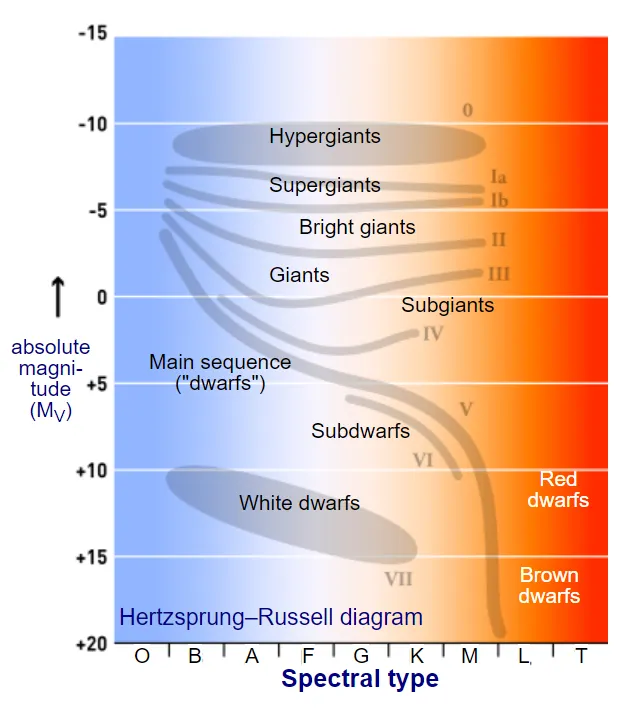
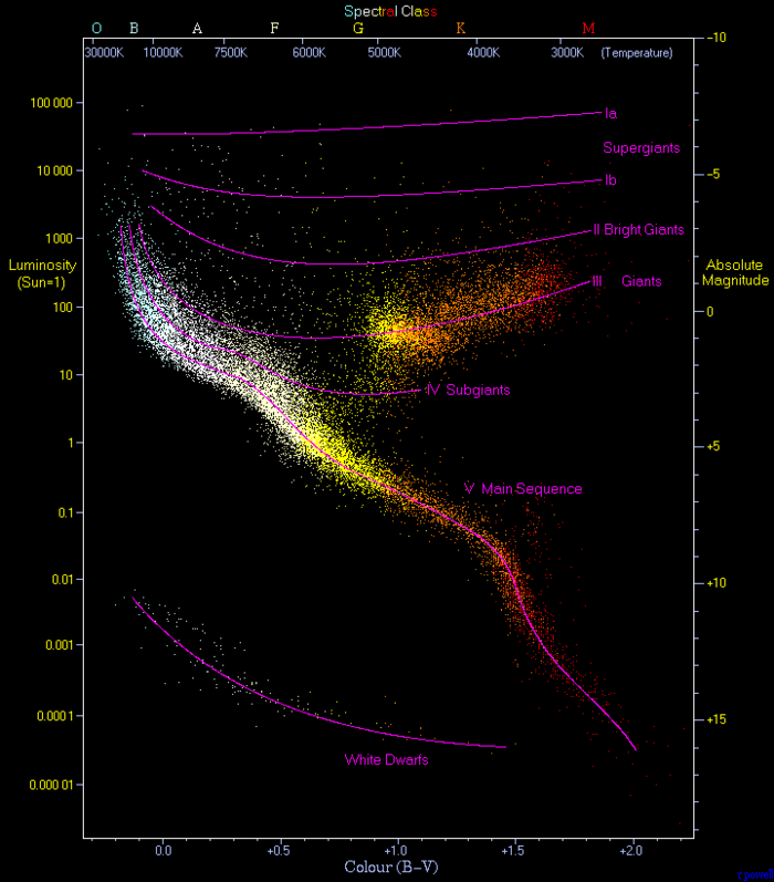
Hertzsprung-Russell Diagram¶

The Hertzsprung-Russell (H-R) diagram is a scatter plot that illustrates the relationship between the luminosity (or absolute magnitude) of stars and their surface temperatures (or spectral classes). It is a fundamental tool in astrophysics for understanding stellar evolution and properties.

The H-R diagram can also show evolutionary tracks of stars, illustrating how they change in luminosity and temperature over time as they evolve through different stages of their life cycles.
The H-R diagram typically has the following features:

Main Sequence: Most stars, including the Sun, fall along a diagonal band called the main sequence. Stars on the main sequence are in a stable phase of hydrogen fusion in their cores. The position of a star on the main sequence is determined by its mass, with more massive stars being hotter and more luminous.
Giants and Supergiants: Above the main sequence, there are regions occupied by giant and supergiant stars. These stars have exhausted the hydrogen in their cores and are in later stages of stellar evolution. They are cooler but much more luminous than main sequence stars of the same temperature.
White Dwarfs: Below the main sequence, there is a region occupied by white dwarfs. These are the remnants of low to intermediate-mass stars that have shed their outer layers. White dwarfs are very hot but have low luminosity due to their small size.

Using the HIPPARCOS dataset, we can plot an H-R diagram by using the absolute magnitude (derived from the apparent magnitude and parallax) against the color index (B-V) to visualize the distribution of stars and their classifications.

Reference¶

Readings¶

Dataset¶

VizieR - Hipparcos Main Catalog