Probability
Probability is calculated and simulated using Python code, typically with libraries like random, numpy, or scipy. Jupyter itself is just the interactive notebook where you run these calculations.
1. Probability Concept
Probability measures how likely an event is to occur.
Formula:
𝑃(𝐸)=
Number of favorable outcomes
Total number of outcomes
P(E)=Total number of outcomes
Number of favorable outcomes
Example: The probability of rolling a 3 on a standard die is:
𝑃(3)=16
P(3)=61
2. Calculating Probability in Python (Jupyter)
You can use Python code in Jupyter to calculate probability. For example:
# Import libraries
import random
# Simulate rolling a die 1000 times
results = [random.randint(1, 6) for _ in range(1000)]
# Probability of rolling a 3
prob_3 = results.count(3) / 1000
print("Estimated probability of rolling a 3:", prob_3)
3. Using numpy or scipy
For more advanced probability calculations:
import numpy as np
from scipy.stats import binom
# Probability of getting exactly 3 heads in 5 coin flips
prob = binom.pmf(3, n=5, p=0.5)
print("Probability of 3 heads:", prob)
binom.pmf(k, n, p) → Probability mass function for binomial events.
Cell In[1], line 12 Example: The probability of rolling a 3 on a standard die is: ^ SyntaxError: invalid non-printable character U+200B
Sample
Coin Tosses simulate
#### import random

# Simulate 1000 coin tosses
tosses = [random.choice(['Heads', 'Tails']) for _ in range(1000)]

# Calculate probabilities
prob_heads = tosses.count('Heads') / 1000
prob_tails = tosses.count('Tails') / 1000

print("Estimated Probability of Heads:", prob_heads)
print("Estimated Probability of Tails:", prob_tails)
import random

# Simulate 1000 coin tosses
tosses = [random.choice(['Heads', 'Tails']) for _ in range(1000)]

# Calculate probabilities
prob_heads = tosses.count('Heads') / 1000
prob_tails = tosses.count('Tails') / 1000

print("Estimated Probability of Heads:", prob_heads)
print("Estimated Probability of Tails:", prob_tails)
Estimated Probability of Heads: 0.524
Estimated Probability of Tails: 0.476
Dice Rolls simulation
# Simulate rolling a 6-sided die 1000 times
dice_rolls = [random.randint(1, 6) for _ in range(1000)]

# Probability of rolling a 3
prob_3 = dice_rolls.count(3) / 1000
print("Estimated Probability of rolling a 3:", prob_3)
Estimated Probability of rolling a 3: 0.172
Visualizing Dice Probabilities
import matplotlib.pyplot as plt

# Count occurrences of each number
counts = [dice_rolls.count(i) for i in range(1,7)]

# Plot bar chart
plt.bar(range(1,7), counts)
plt.xlabel('Dice Number')
plt.ylabel('Frequency')
plt.title('Dice Roll Simulation')
plt.show()

Binomial Distribution
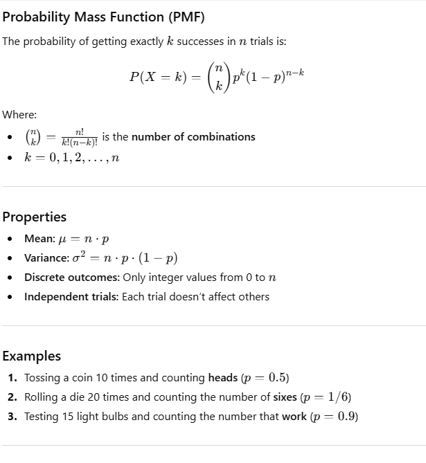
- The binomial distribution models the number of successes in a fixed number of independent trials, where each trial has only two possible outcomes:
Success (with probability p) Failure (with probability 1−p)
It is defined by two parameters: n = number of trials p = probability of success in a single trial
Probability Mass Function (PMF)
The probability of getting exactly 𝑘k successes in 𝑛 n trials is:
Probability
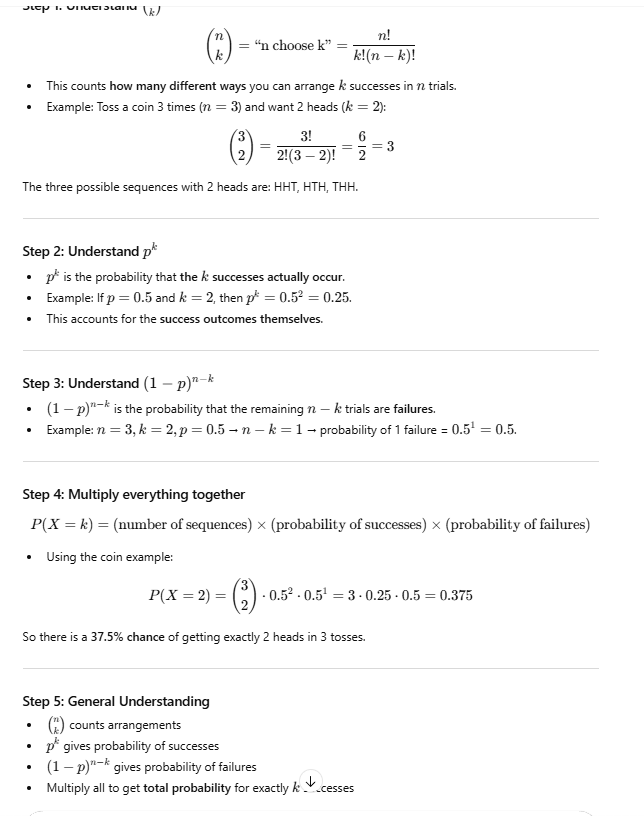
Explaination of the Binomialprobability formula in deatils. I want to know each formula in detal
import itertools
import matplotlib.pyplot as plt

# Parameters
n = 3          # number of trials
p = 0.5        # probability of success
k = 2          # number of successes

# Step 1: Generate all sequences of successes (H) and failures (T)
trials = ['H', 'T']
sequences = list(itertools.product(trials, repeat=n))

# Step 2: Count sequences with exactly k successes
valid_sequences = [seq for seq in sequences if seq.count('H') == k]

# Step 3: Calculate probability
prob = len(valid_sequences) * (p**k) * ((1-p)**(n-k))

# Step 4: Display results
print(f"All possible sequences ({len(sequences)} total):")
for seq in sequences:
    print(seq)

print("\nSequences with exactly 2 successes:")
for seq in valid_sequences:
    print(seq)

print(f"\nP(X={k}) = {prob}")

# Step 5: Visualize sequences
colors = ['green' if seq.count('H')==k else 'lightgray' for seq in sequences]

plt.figure(figsize=(8,4))
plt.bar(range(len(sequences)), [1]*len(sequences), color=colors)
plt.xticks(range(len(sequences)), [''.join(seq) for seq in sequences])
plt.ylabel("Probability weight (conceptual)")
plt.title(f"Binomial Distribution Visualization (n={n}, k={k})\ngreen = sequences with exactly {k} successes")
plt.show()
All possible sequences (8 total):
('H', 'H', 'H')
('H', 'H', 'T')
('H', 'T', 'H')
('H', 'T', 'T')
('T', 'H', 'H')
('T', 'H', 'T')
('T', 'T', 'H')
('T', 'T', 'T')

Sequences with exactly 2 successes:
('H', 'H', 'T')
('H', 'T', 'H')
('T', 'H', 'H')

P(X=2) = 0.375

Explanation of Visualization Each bar represents one possible sequence of trials. Green bars = sequences with exactly k successes. Probability formula: P(X=k) = \underbrace{\text{# of green sequences}}_{\binom{n}{k}} \cdot p^k \cdot (1-p)^{n-k}
This makes it very clear how the formula combines “arrangements × success probability × failure probability”.
from IPython.display import display, Math

display(Math(r'P(E) = \frac{\text{Number of favorable outcomes}}{\text{Total number of outcomes} }'))
display(Math(r'P(E^c) = 1 - P(E)'))
display(Math(r'P(A \cup B) = P(A) + P(B) - P(A \cap B)'))
display(Math(r'P(X=k) = \binom{n}{k} p^k (1-p)^{n-k}'))
import numpy as np
import matplotlib.pyplot as plt
from scipy.stats import binom, norm

# Binomial Distribution
n, p = 10, 0.5
x = np.arange(0, n+1)
prob = binom.pmf(x, n, p)
plt.bar(x, prob, color='skyblue')
plt.title("Binomial Distribution (n=10, p=0.5)")
plt.show()

# Normal Distribution
mu, sigma = 0, 1
x = np.linspace(-4, 4, 1000)
plt.plot(x, norm.pdf(x, mu, sigma), color='red')
plt.title("Normal Distribution (μ=0, σ=1)")
plt.show()


Students mark
import numpy as np

# Example marks of 20 students
marks = [55, 70, 80, 90, 65, 75, 85, 60, 50, 95, 88, 72, 78, 82, 68, 90, 77, 66, 84, 91]
Frequency Distribution
# Define bins (intervals) for marks
bins = [0, 50, 60, 70, 80, 90, 100]

# Count number of students in each bin
freq, bin_edges = np.histogram(marks, bins=bins)

print("Frequency:", freq)
print("Bins:", bin_edges)
Frequency: [0 2 4 5 5 4]
Bins: [  0  50  60  70  80  90 100]
Calculate probabilities
probabilities = freq / len(marks)
print("Probabilities:", probabilities)
Probabilities: [0. 0.1 0.2 0.25 0.25 0.2 ]
Visualize probability distribution
import matplotlib.pyplot as plt

# Midpoint of each bin for plotting
mid_points = (bin_edges[:-1] + bin_edges[1:]) / 2

plt.bar(mid_points, probabilities, width=8, color='skyblue', edgecolor='black')
plt.xlabel("Marks Range")
plt.ylabel("Probability")
plt.title("Probability Distribution of Students' Marks")
plt.show()

Cumulative Probability
cumulative_prob = np.cumsum(probabilities)
print("Cumulative Probabilities:", cumulative_prob)

plt.plot(mid_points, cumulative_prob, marker='o', color='red')
plt.xlabel("Marks Range")
plt.ylabel("Cumulative Probability")
plt.title("Cumulative Probability of Students' Marks")
plt.grid(True)
plt.show()
Cumulative Probabilities: [0. 0.1 0.3 0.55 0.8 1. ]

✅ Explanation
Histogram bins → divide marks into intervals (like 50–60, 60–70…).
Frequency → number of students in each bin.
Probability → frequency divided by total students.
Visualization: bar chart for probability, line chart for cumulative probability