FAB Futures - Data Science

Home About

Data Science/Session 5 > Probability

The second session in a row that left me dizzy. I felt like I was on one of those playground 'spinners' and Neil was the kid in charge of spinning it faster and faster. I did my best to hang on for as long as possible and was surprised that I was able to keep pace for about 80% of the class...before I was overwhelmed by mathematical terminology and equations.

But last week's work has instilled me with some confidence. The Machine Learning session a few days ago also left me equally confused, but by the end of the assignment week not only did I feel that I was able to get achieve basic understanding of the material...but I actually had fun in the learning process!! Admittedly there was A LOT of grunt work involved...learning new terminology and concepts one-by-one, studying code line-by-line. But all that effort paid off, as I managed to build a Machine Learning model to recognize Japanese Numerals.

What I learned from last week's procedure was that a obvious path towards the objective may not be the most efficient way. Confused by the many new words and processes, a logical path may have been to get an understanding of those things first. Instead, I chose to follow a guide and go down down a side path, to dive right in and just start building a Machine Learning model from scratch. What made all the difference was finding a great series of tutorial videos on YouTube that walked me through each step of the process. As I followed instructions and built my model in emulation of the example piece-by-piece, I was introduced to and learned those confusing terms and procedures that Neil shared one-by-one and in a logical, pragmatic way. I suppose this was an example of learn by doing rather than learning theory and concepts. Anyhow, I am thinking to take this same approach in this week, to get past the fog of knowledge and learn by gettin my hands dirty.

Research

• Dissecting Neil's Programs
• Technical Analysis

Assignment

Learning to build a Machine Learning model to recognize characters was fun last week. This week, I return back to my original dataset...NVIDIA's stock data.

When I worked as a Security Analyst on Wall Street, I was trained as a Fundamental Analyst. What this meant was that I looked at financial and non-financial information about a company, and used them to make Quantitative (calculations) and Qualitative (observations and assessments) analysis and conclusions. I built spreadsheets to assess the current condition of financial statements and other business metrics, as well as made predictions of how financial and business metrics may trend going forward into the future. And these predictions led to conclusions and recommendations about whether to buy, hold or sell a stock.

In contrast to Fundamental Analysts were Technical Analysts, those who did little of what I just described (I assumed), but made buy, hold and sell decision based on trend observations of charts and plots for different companies. I am probably grossly oversimplifying the difference, but my understand of the work of Technical Analysts is that they relied heavily on statistical analysis to make their stock decisions.

Twelve, Twenty Six, Nine

Last session's learning content reminded me of the tools used by Technical Analysts. And when I Googled "stock histogram", I was introduced to the MACD. According to Investopedia, MACD is an acronym for Moving Average Convergence Divergence..."a tool that helps technical traders spot changes in market momentum and trend reversals." The website alpharithms provides this MACD formula

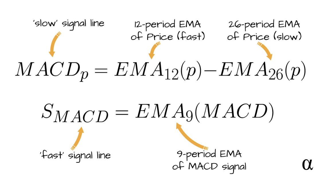
...and additional explanations regarding MACD:

• MACD..."is a momentum indicator that describes **shifts in values over several periods of time-series"
• *"is made of several distinct exponential moving averages (EMA) calculations made across different periods of observation
• "produces the MACD line, the Signal Line, and a value signifying the Convergence/Divergence between them."
• "These values are often visualized as a chart of two signal lines plotted to overlay a histogram"

So to satisfy this session's assignment, I am thinking to build a MACD indicator in Python.

I found this tutorial on YouTube called Building a MACD Indicator in Python. Let's see what we can learn!!

! pip install yfinance

# MACD Histogram > Nvidia

# import yahoo finance library
import yfinance as yf

# pull stock data from yahoo finance
nvda = yf.Ticker('NVDA') #specify stock ticker, assign to a variable
data = nvda.history(interval="1h", period="60d") #pull historical data, specify interval and period
data #show data

	Open	High	Low	Close	Volume	Dividends	Stock Splits
Datetime
2025-09-10 09:30:00-04:00	176.649994	178.949997	175.479996	177.649994	82319968	0.0	0.0
2025-09-10 10:30:00-04:00	177.649994	179.289993	177.600006	178.614197	36684204	0.0	0.0
2025-09-10 11:30:00-04:00	178.619995	178.729996	177.479996	177.990005	20946072	0.0	0.0
2025-09-10 12:30:00-04:00	177.979996	178.149994	177.369995	178.005096	14456545	0.0	0.0
2025-09-10 13:30:00-04:00	178.005005	178.320007	176.149994	176.274994	18519526	0.0	0.0
...	...	...	...	...	...	...	...
2025-12-03 11:30:00-05:00	180.544998	181.220001	179.820007	180.375000	10736030	0.0	0.0
2025-12-03 12:30:00-05:00	180.369995	180.979996	180.064499	180.649994	7611606	0.0	0.0
2025-12-03 13:30:00-05:00	180.660004	181.279999	180.442093	180.744995	9127929	0.0	0.0
2025-12-03 14:30:00-05:00	180.744095	180.960007	179.910004	180.020004	10015000	0.0	0.0
2025-12-03 15:30:00-05:00	180.020004	180.029999	179.279999	179.639999	49322097	0.0	0.0

416 rows × 7 columns

Wow! The Yahoo! Finance extension made pulling stock data for analysis super easy! No more scouring the internet looking for data downloads. That alone made this tutorial worth something.

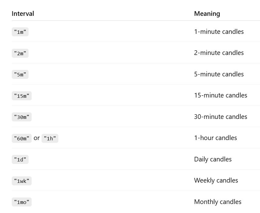
According to ChatGPT, the parameter parameter options for the 'history' command is as follows:

Interval Options

Period Options

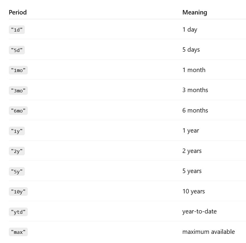
I chose 1-hour price data over a 60 days period.

# Create MACD 12 and 26 Period EMA Dataframe entries
# 12 = sensitive to short-term price movement
# 26 = a longer term trend

data['EMA12'] = data['Close'].ewm(span=12, adjust=False).mean()  # pandas EWM = exponentially weighted movement, mean to calc avg
data['EMA26'] = data['Close'].ewm(span=26, adjust=False).mean()

# Calculate MACD
data['MACD'] = data['EMA12'] - data['EMA26']

# Calculate the Signal Line 9 Period EMA
data['Signal_Line'] = data['MACD'].ewm(span=9, adjust=False).mean()

data

	Open	High	Low	Close	Volume	Dividends	Stock Splits	EMA12	EMA26	MACD	Signal_Line
Datetime
2025-09-10 09:30:00-04:00	176.649994	178.949997	175.479996	177.649994	82319968	0.0	0.0	177.649994	177.649994	0.000000	0.000000
2025-09-10 10:30:00-04:00	177.649994	179.289993	177.600006	178.614197	36684204	0.0	0.0	177.798333	177.721416	0.076916	0.015383
2025-09-10 11:30:00-04:00	178.619995	178.729996	177.479996	177.990005	20946072	0.0	0.0	177.827821	177.741312	0.086509	0.029608
2025-09-10 12:30:00-04:00	177.979996	178.149994	177.369995	178.005096	14456545	0.0	0.0	177.855094	177.760851	0.094243	0.042535
2025-09-10 13:30:00-04:00	178.005005	178.320007	176.149994	176.274994	18519526	0.0	0.0	177.612002	177.650788	-0.038786	0.026271
...	...	...	...	...	...	...	...	...	...	...	...
2025-12-03 11:30:00-05:00	180.544998	181.220001	179.820007	180.375000	10736030	0.0	0.0	180.653862	180.332579	0.321283	0.294286
2025-12-03 12:30:00-05:00	180.369995	180.979996	180.064499	180.649994	7611606	0.0	0.0	180.653267	180.356091	0.297176	0.294864
2025-12-03 13:30:00-05:00	180.660004	181.279999	180.442093	180.744995	9127929	0.0	0.0	180.667379	180.384899	0.282480	0.292387
2025-12-03 14:30:00-05:00	180.744095	180.960007	179.910004	180.020004	10015000	0.0	0.0	180.567783	180.357869	0.209913	0.275892
2025-12-03 15:30:00-05:00	180.020004	180.029999	179.279999	179.639999	49322097	0.0	0.0	180.425047	180.304694	0.120353	0.244784

416 rows × 11 columns

Great! Both the MACD and the Signal Line values have been calculated. Now we need the Convergence/Divergence value.

We will need 4 terms for the calculation > the most recent MACD and Signal Line values, as well as the next previous MACD and Signal Line values.

last_row = data.iloc[-1] # data index location -1
second_last_row = data.iloc[-2] # data index location -2

print(f"last_row MACD: {last_row['MACD']}")
print(f"last_row Signal_Line: {last_row['Signal_Line']}")
print(f"second_last_row MACD: {second_last_row['MACD']}")
print(f"second_last_row Signal_Line: {second_last_row['Signal_Line']}")

last_row MACD: 0.12035281205442061
last_row Signal_Line: 0.2447842657560711
second_last_row MACD: 0.20991313019459312
second_last_row Signal_Line: 0.2758921291814837

if second_last_row['MACD'] > second_last_row['Signal_Line'] and last_row['MACD'] < last_row['Signal_Line']:
    print('cross below')

elif second_last_row['MACD'] < second_last_row['Signal_Line'] and last_row['MACD'] > last_row['Signal_Line']:
    print('cross above')

else:
    print('no crossover')

no crossover

Almost, but not quite there. The tutorial ended abruptly after only showing how to pull data from Yahoo! Finance, create a dataframe and do some math in Python. Learned a few things but...no Histogram. No Fit Function.

Next...

Let's see if this tutorial Python Tutorial. MACD Stock Technical Indicator gets us closer.

• "Moving averages convergence/divergence MACD consists of centered oscillator that measures a stock's price momentum and identifies trends. 12 days are commonly used for short term smoothing, 26 days fo long term smoothing and 9 days for signal" Gerald Appel

Calculations

• MACD Indicator Calculation > MACD(12,26) = EMA12(Close) - EMA26(Close)
• 9 days MACD Indicator Signal Calculation > Signal(9) = EMA9[MACD(12,26)]
• MACD Indicator Histogram calculation > MACD Histogram(12,26,9) = MACD(12,26) - Signal(9)

The tutorial calls for the installation of the TA-lib library...or Technical Analysts library...presumably with custom methods to make technical analysis calculations easier. I could just PIP install it. Papayita!!

! pip install TA-lib

! pip install pandas

! pip install matplotlib

# Import Libraries

import numpy as np
import pandas as pd
import matplotlib.pyplot as plt
import talib as ta

# MACD Histogram > Nvidia

# import yahoo finance library
import yfinance as yf

# pull stock data from yahoo finance
nvda = yf.Ticker('NVDA') #specify stock ticker, assign to a variable
data = nvda.history(interval="1d", period="5y") #pull historical data, specify interval and period
data #show data

	Close	High	Low	Open	Volume	Dividends	Stock Splits
Date
2020-12-03 00:00:00-05:00	NaN	NaN	NaN	NaN	0	0.004	0.0
2020-12-04 00:00:00-05:00	13.520983	13.522728	13.351948	13.411534	202244000	0.000	0.0
2020-12-07 00:00:00-05:00	13.569347	13.693505	13.462891	13.563863	223244000	0.000	0.0
2020-12-08 00:00:00-05:00	13.313305	13.561371	13.244993	13.547659	271920000	0.000	0.0
2020-12-09 00:00:00-05:00	12.895205	13.377127	12.832877	13.263939	401300000	0.000	0.0
...	...	...	...	...	...	...	...
2025-11-26 00:00:00-05:00	180.259995	182.910004	178.240005	181.630005	183852000	0.000	0.0
2025-11-28 00:00:00-05:00	177.000000	179.289993	176.500000	179.009995	121332800	0.000	0.0
2025-12-01 00:00:00-05:00	179.919998	180.300003	173.679993	174.759995	188131000	0.000	0.0
2025-12-02 00:00:00-05:00	181.460007	185.660004	180.000000	181.759995	182632200	0.000	0.0
2025-12-03 00:00:00-05:00	179.589996	182.449997	179.110001	181.080002	164721400	0.000	0.0

1256 rows × 7 columns

# MACD Stock Technical Indicator
data['MACD'], data['MACDsig'], data['MACDhist'] = ta.MACD(
    np.asarray(data['Close']),
    fastperiod=12,
    slowperiod=26,
    signalperiod=9
)
data

	Close	High	Low	Open	Volume	Dividends	Stock Splits	MACD	MACDsig	MACDhist
Date
2020-12-03 00:00:00-05:00	NaN	NaN	NaN	NaN	0	0.004	0.0	NaN	NaN	NaN
2020-12-04 00:00:00-05:00	13.520983	13.522728	13.351948	13.411534	202244000	0.000	0.0	NaN	NaN	NaN
2020-12-07 00:00:00-05:00	13.569347	13.693505	13.462891	13.563863	223244000	0.000	0.0	NaN	NaN	NaN
2020-12-08 00:00:00-05:00	13.313305	13.561371	13.244993	13.547659	271920000	0.000	0.0	NaN	NaN	NaN
2020-12-09 00:00:00-05:00	12.895205	13.377127	12.832877	13.263939	401300000	0.000	0.0	NaN	NaN	NaN
...	...	...	...	...	...	...	...	...	...	...
2025-11-26 00:00:00-05:00	180.259995	182.910004	178.240005	181.630005	183852000	0.000	0.0	-2.466982	-0.747131	-1.719851
2025-11-28 00:00:00-05:00	177.000000	179.289993	176.500000	179.009995	121332800	0.000	0.0	-2.853962	-1.168497	-1.685464
2025-12-01 00:00:00-05:00	179.919998	180.300003	173.679993	174.759995	188131000	0.000	0.0	-2.891692	-1.513136	-1.378556
2025-12-02 00:00:00-05:00	181.460007	185.660004	180.000000	181.759995	182632200	0.000	0.0	-2.765450	-1.763599	-1.001851
2025-12-03 00:00:00-05:00	179.589996	182.449997	179.110001	181.080002	164721400	0.000	0.0	-2.784202	-1.967720	-0.816482

1256 rows × 10 columns

# price chart
fig1, ax = plt.subplots(2, sharex=True)
ax[0].plot(data['Close'], label='Close Price')
ax[0].legend(loc='upper left')

# MACD chart
ax[1].plot(data['MACD'], label='MACD')
ax[1].plot(data['MACDsig'], label='Signal Line')
ax[1].plot(data['MACDhist'], linestyle='--', label='Histogram')
ax[1].legend(loc='upper left')

plt.suptitle('NVDA Close Prices and MACD(12,26,9) Stock Technical Iindicator')
plt.show()

OK...it is an improvement over the last tutorial. At least I have some graphs to show for it. Because the second tutorial used a proprietary dataset in .CSV format that I didn't have access to, I used code from the first tutorial to pull the stock price data for Nvidia from Yahoo! finance...and actually got it to work. ChatGPT gave me a hand with adding legends after I received the error "No artists with labels found". Hooray!

Matplotlib was used to generate the charts...but the histogram line LOOKS STRANGE. Shouldn't it be a bell-shaped distribution? Are negative numbers allowed?

I asked ChatGPT to make the Histogram into bar charts and to add a zero line. Here is the resulting code.

fig1, ax = plt.subplots(2, sharex=True, figsize=(12, 7)) #chatGPT added 'figsize'

# Price chart
ax[0].plot(data['Close'], label='Close Price')
ax[0].legend(loc='upper left')

# --- MACD section ---
# MACD line
ax[1].plot(data['MACD'], label='MACD', linewidth=1.2) #chatGPT added 'linewidth'

# Signal line
ax[1].plot(data['MACDsig'], label='Signal Line', linewidth=1.2) #chatGPT added 'linewidth'

# Histogram bars
ax[1].bar(data.index, data['MACDhist'], 
          label='Histogram',
          color='black', alpha=0.7) #chatGPT added 'color' and 'alpha'

# Zero line
ax[1].axhline(0, color='grey', linewidth=1) #chatGPT added 'axhline'

ax[1].legend(loc='upper left')
plt.suptitle('NVDA Close Prices and MACD(12,26,9)')
plt.show()

Dang it! I asked ChatGPT "Are stock histogram charts the same as a statistical histogram charts?". The answer was a resounding..."NO!"

MACD Histogram is not a true Histogram. Doh!

"It is a time-series bar data where each bar corresponds to one time period (day, minute, etc.)"

**MACD Histograms fails to:

• group anything into bins
• not based on frequency counts
• have only positive values
• x-axis is 'Time' not 'Values'

So the MACD experiment was a...FAIL!!

Back to ChatGPT with the question "can a statistical histogram be used with stock historical data?"

The Answer: "Yes — absolutely! A statistical histogram is very useful with stock historical data. You just need to use the right type of stock data."

• Histogram of Daily Returns
• Histogram of Log Returns
• Histogram of Daily Price Changes
• Histogram of Daily Trading Volume
• Histogram of Volatility
• Histogram of the Indicators (MACD, RSI) themselves

But...'Closing Price' should not be used as data for Statistical Histogram analysis...nothing useful would result as stock prices trend and are heavily skewed.

"Histograms are used for analyzing distribution not trends"

So I asked ChatGPT to show me a Statistical Analysis Histogram for a stock's Daily Trading Volume, and it offered this up...

# Example of Stock Trading Volume Histogram
# by ChatGPT

import matplotlib.pyplot as plt
import numpy as np

# Percent change in volume
data['VolChange'] = data['Volume'].pct_change()

# Replace +/- inf with NaN, then drop them
vol_change_clean = data['VolChange'].replace([np.inf, -np.inf], np.nan).dropna()

plt.figure(figsize=(10, 5))
plt.hist(vol_change_clean, bins=50, edgecolor='black')
plt.plot(data['Volume'],0*data['Volume'],'|',ms=npts/20)

plt.title("Histogram of Volume Percent Changes")
plt.xlabel("Percent Change")
plt.ylabel("Frequency")
plt.show()

GREAT!! Now THAT looks more like a proper Histogram. A distribution with a long tail.

The Observation > Over the pass 60 days, Nvidia's trading volume basically didn't change much...hovering around zero percent change.

So looking at the code, I see that ChatGPT:

• loads 2 libraries > matplotlib and numpy
• calculate the percentage change in volume using the 'pct_change()' command
• a calculation to clean data by dropping zero values and preventing infinite values from causing trouble in the next steps
• set the plot figure size with the 'figure' command
• plot the histogram with the 'hist' command
• plot title and labels
• show everything with the 'show()' command

Looks pretty simple. All I have to do is feed the program the right 'Volume' data!

I want to plot the Gaussian (normal) line on top of the histogram so asked ChatGPT 'modify the code to add gaussian line". Here is what it returned...

# Example of Stock Trading Volume Histogram with Gaussian Fit
# by ChatGPT

import matplotlib.pyplot as plt
import numpy as np

# Percent change in volume
data['VolChange'] = data['Volume'].pct_change()

# Replace +/- inf with NaN, then drop them
vol_change_clean = data['VolChange'].replace([np.inf, -np.inf], np.nan).dropna()

# Compute mean and standard deviation for Gaussian
mu = vol_change_clean.mean()
sigma = vol_change_clean.std()

plt.figure(figsize=(10, 5))

# Use density=True so histogram area = 1, matching the Gaussian PDF scale
count, bins, _ = plt.hist(vol_change_clean, bins=50, 
                          alpha=0.6, density=True, label='Histogram')

# Create x values covering the range of the data
x = np.linspace(bins[0], bins[-1], 500)

# Gaussian (normal) probability density function
gaussian = (1 / (sigma * np.sqrt(2 * np.pi))) * np.exp(-0.5 * ((x - mu) / sigma) ** 2)

# Plot the Gaussian line
plt.plot(x, gaussian, linewidth=2, label='Gaussian Fit')

plt.title("Histogram of Nvidia Trading Volume (5yr)")
plt.xlabel("Percent Change")
plt.ylabel("Density")
plt.legend()
plt.show()

It added:

• calculations for mu by means of the mean() method
• calculations for sigma by means of the std() (standard deviation) method
• calculated x values for the data range using the linspace() method
• calculated the gaussian (y) value
  also...
• set density to 'True' in the hist() method to allow Gaussian and Histogram to share the same graph scale
• plot the Gaussian Fit line

I deleted edgecolor to remove the black outline around the bars and change the name of the chart to "Histogram of NVDA Trading Volume (5yr)"

The Observation > the fit function confirms that Nvidia's trading volume did indeed hover around zero percent change...but is skewed slightly to the positive change side (not slightly negative as suggested visually by the histogram itself).

Let's see if the program is basically the same if I ask it to give me a program to create a histogram for 'Volatility' (the code should mostly be very similar except for the calculations section).

# Statistical Histogram of Stock Volatility (Rolling 20-day)
# by ChatGPT

import pandas as pd
import numpy as np
import matplotlib.pyplot as plt

# 1. Compute log returns
data['LogReturn'] = np.log(data['Close'] / data['Close'].shift(1))

# 2. Compute 20-day rolling volatility (annualized)
data['Volatility20'] = data['LogReturn'].rolling(20).std() * np.sqrt(252)

# Clean data
vol = data['Volatility20'].dropna()

# --- Compute Gaussian parameters ---
mu = vol.mean()
sigma = vol.std()

# --- Plot histogram (density=True so Gaussian fits scale) ---
plt.figure(figsize=(10, 10))
count, bins, _ = plt.hist(vol, bins=50, density=True, alpha=0.6, label='Volatility Histogram')

# --- Create x-range for Gaussian curve ---
x = np.linspace(bins[0], bins[-1], 500)

# --- Gaussian Probability Density Function ---
gaussian = (1 / (sigma * np.sqrt(2 * np.pi))) * np.exp(-0.5 * ((x - mu) / sigma)**2)

# --- Overlay Gaussian line ---
plt.plot(x, gaussian, linewidth=2, label='Gaussian Fit')

# Labels and title
plt.title("Histogram Nvidia 20-Day Rolling Volatility (Annualized)")
plt.xlabel("Volatility")
plt.ylabel("Density")
plt.legend()

plt.show()

Let me see if I understand the code...

• Import 3 libraries this time > pandas, in addition to numpy and matplotlib
• Calculate Log Returns using the stock's 'Closing Price' divided by the closing price of the previous day
• Calculate the '20-day Rolling Volatility' of the Log Returns by running the 'std()' command on it
• Clean data...removing zero values (I think)
• Calculated Mu and Sigma
• Set Histogram density value to 'true'
• Calculate the x-range for Gaussian assign to variable 'x'
• Calculate Gaussian values (y-values)

...as before with the Volume Histogram, go through the steps to plot the chart.

Interesting that while the bar graph DID NOT generate a Bell-shaped, normal distribution (I asked ChatGPT about this and it said that it is not uncommon), but the Gaussian Fit line clearly shows the peak volatility value (approximately 0.5). This was a surprised, as the Histogram showed several peaks and valleys (which made me think that I again did something wrong and didn't get a proper histogram plot).

So the value of generating and plotting a Fit Function becomes clear...as it reveals and makes clear the hidden trend in the data!!

OK!! Bare minimum assignment work done!!

Next!!!...let's tackle another probability algorithm!

Learning Outcome

• The word 'Histogram' can mean many things. Technical Analysts call 'Time Series Bar Charts' as Histograms...but are NOT the same as Statistical Histograms that we were asked to learn.
• (still processing...)

Definitions (WIP)

Lots of new and mysterious terms this session!! I think it is best that I gain some basic understanding of them, to get the most out of the session.

Probability - Unconditional, Joint, Conditional

Bayesian

Likelihood

Prior

Evidence

Gaussian > distribution type with a bell-shape

Central Limit Theorem

Histogram

Mean

Standard Deviation

Variance

Co-variance

Averaging > distribution on the distribution

Multi-Dimensional Distribution

Entropy

Mutual Information