Research > Expectation Maximization
Tutorial 1
EM Algorithm in Machine Learning
Latent Variables for Maximum Likelihood
- how to estimate the joint probability distribution for a dataset
- "Probability Density Estimation is the construction of an estimate based on observed data, involving the selection of a probability distribution function and the parameters of that function that best explains the joint probability of the observed data."
import matplotlib.pyplot as plt
import numpy as np
from numpy.random import normal
np.random.seed(0) # seed number 0
sample = normal(size=2000)
plt.hist(sample,bins=100) # number of bins is important
(array([ 2.,  0.,  0.,  2.,  3.,  0.,  2.,  3.,  2.,  1.,  2.,  1.,  4.,
         3.,  4.,  3.,  6.,  8.,  2., 10., 13., 11., 21., 16., 13., 21.,
        20., 20., 15., 22., 26., 25., 31., 37., 32., 43., 42., 36., 43.,
        33., 43., 47., 51., 51., 48., 39., 47., 51., 53., 67., 48., 47.,
        61., 43., 45., 55., 45., 47., 37., 31., 26., 38., 34., 35., 39.,
        29., 23., 19., 13., 18., 22., 22., 15., 15., 13., 10., 15., 11.,
         7.,  9.,  8.,  7.,  1.,  7.,  5.,  6.,  4.,  3.,  1.,  4.,  1.,
         2.,  2.,  1.,  0.,  0.,  0.,  0.,  0.,  1.]),
 array([-3.04614305e+00, -2.98397188e+00, -2.92180070e+00, -2.85962952e+00,
        -2.79745834e+00, -2.73528716e+00, -2.67311599e+00, -2.61094481e+00,
        -2.54877363e+00, -2.48660245e+00, -2.42443127e+00, -2.36226009e+00,
        -2.30008892e+00, -2.23791774e+00, -2.17574656e+00, -2.11357538e+00,
        -2.05140420e+00, -1.98923302e+00, -1.92706185e+00, -1.86489067e+00,
        -1.80271949e+00, -1.74054831e+00, -1.67837713e+00, -1.61620595e+00,
        -1.55403478e+00, -1.49186360e+00, -1.42969242e+00, -1.36752124e+00,
        -1.30535006e+00, -1.24317888e+00, -1.18100771e+00, -1.11883653e+00,
        -1.05666535e+00, -9.94494172e-01, -9.32322993e-01, -8.70151815e-01,
        -8.07980637e-01, -7.45809458e-01, -6.83638280e-01, -6.21467102e-01,
        -5.59295924e-01, -4.97124745e-01, -4.34953567e-01, -3.72782389e-01,
        -3.10611210e-01, -2.48440032e-01, -1.86268854e-01, -1.24097676e-01,
        -6.19264973e-02,  2.44680964e-04,  6.24158592e-02,  1.24587038e-01,
         1.86758216e-01,  2.48929394e-01,  3.11100572e-01,  3.73271751e-01,
         4.35442929e-01,  4.97614107e-01,  5.59785285e-01,  6.21956464e-01,
         6.84127642e-01,  7.46298820e-01,  8.08469999e-01,  8.70641177e-01,
         9.32812355e-01,  9.94983533e-01,  1.05715471e+00,  1.11932589e+00,
         1.18149707e+00,  1.24366825e+00,  1.30583942e+00,  1.36801060e+00,
         1.43018178e+00,  1.49235296e+00,  1.55452414e+00,  1.61669532e+00,
         1.67886649e+00,  1.74103767e+00,  1.80320885e+00,  1.86538003e+00,
         1.92755121e+00,  1.98972239e+00,  2.05189356e+00,  2.11406474e+00,
         2.17623592e+00,  2.23840710e+00,  2.30057828e+00,  2.36274946e+00,
         2.42492063e+00,  2.48709181e+00,  2.54926299e+00,  2.61143417e+00,
         2.67360535e+00,  2.73577653e+00,  2.79794770e+00,  2.86011888e+00,
         2.92229006e+00,  2.98446124e+00,  3.04663242e+00,  3.10880360e+00,
         3.17097477e+00]),
 <BarContainer object of 100 artists>)

Questions: Which probability distribution function to choose? How to choose the parameters for that function?
Solution: "Maximum Likelihood Estimation Algorithm = the method of estimating the parameters of a probability distribution by maximizing the likelihood function in order to make the observed data most probable for the statistical model"
Limitation: "Assumes the data is completely and fully observed and all variables relevant to the model are already present. But sometimes some variables remain hidden (Latent Variables) and cause inconsistencies."
Another Solution: *"Expectation Maximization Algorithm = finding appropriate distribution parameters in the presence of Latent Variables.
EM Algorithm In Machine Learning
"EM Algorithm is used to find the local maximum likelihood parameters of a statistical mode, in case Latent Variables are present or the dataset is incomplete."
The Procedure:
- Consider a set of Starting Parameters in the incomplete data
- Expectation Step to estimate the missing values in the data, using the observed data to guess the missing values.
3.Maximization Step generates complete data by updating the missing value in the data - Repeat steps 2 & 3...until Convergence (based on intuition, when 2 random variables and the probability of their difference is very small...if the values match each other) is met
How does EM Algorithm Work
- Use Observed Data to estimate the missing data and then updating those values of parameter
- A set of initial parameters is considered
- A set of unobserved and incomplete data is given to the system
- ...with an assumption that the observed data is coming from a specific model
- Next the Expectation step (E-step)
- Use the observed data to estimate the missing or incomplete value or data
- Next the Maximization step (M-step) used to complete the data generated in the e-step...updates the hypothesis
- Then Convergence Check
Gaussian Mixture Model
"Gaussian Mixture Model (GMM) is a model that uses a combination of probability distributions and and require the estimation of mean and standard deviation parameters"
- Maximum Likelihood Estimation the most common method for estimating parameters for the GMM
Case: data points are generated by 2 different processes and each process has a Gaussian probability distribution...but unclear as to which distribution a given data point belongs to

- In EM algo, the e-step estimates the expected value for each Latent Variable
- The m-step would optimize the parameters of the distribution using the maximum likelihood
A new program to run the described case...
# import needed libraries
from numpy import hstack
from numpy.random import normal
import matplotlib.pyplot as plt
# create 2 data point samples, different location and size
sample1 = normal(loc=20, scale=5, size=4000)
sample2 = normal(loc=40, scale=5, size=8000)
# combine 2 samples into 1 with hstack command
sample = hstack((sample1, sample2))
plt.hist(sample, bins=50,density=True) # density = true to change y-axis to probability density, not raw counts
(array([7.03577536e-05, 1.40715507e-04, 7.03577536e-05, 0.00000000e+00,
        7.03577536e-05, 4.92504275e-04, 1.40715507e-03, 2.60323688e-03,
        3.16609891e-03, 5.41754703e-03, 7.24684862e-03, 1.13979561e-02,
        1.46344127e-02, 1.87855202e-02, 2.27255544e-02, 2.27959122e-02,
        2.71580929e-02, 2.53287913e-02, 2.46252138e-02, 2.50473603e-02,
        2.01926753e-02, 1.57601368e-02, 1.30865422e-02, 1.04129475e-02,
        1.00611588e-02, 1.06240208e-02, 1.45640550e-02, 1.68155031e-02,
        2.27255544e-02, 3.27867132e-02, 3.76413982e-02, 4.34107340e-02,
        4.78432724e-02, 5.38236815e-02, 5.30497462e-02, 5.29090307e-02,
        4.54511088e-02, 3.49678035e-02, 2.82838169e-02, 2.27255544e-02,
        1.58304946e-02, 1.16090293e-02, 6.96541761e-03, 3.37717217e-03,
        3.30681442e-03, 1.40715507e-03, 9.14650797e-04, 2.11073261e-04,
        2.11073261e-04, 1.40715507e-04]),
 array([-0.14568943,  1.03873346,  2.22315634,  3.40757922,  4.59200211,
         5.77642499,  6.96084787,  8.14527075,  9.32969364, 10.51411652,
        11.6985394 , 12.88296228, 14.06738517, 15.25180805, 16.43623093,
        17.62065382, 18.8050767 , 19.98949958, 21.17392246, 22.35834535,
        23.54276823, 24.72719111, 25.91161399, 27.09603688, 28.28045976,
        29.46488264, 30.64930553, 31.83372841, 33.01815129, 34.20257417,
        35.38699706, 36.57141994, 37.75584282, 38.9402657 , 40.12468859,
        41.30911147, 42.49353435, 43.67795724, 44.86238012, 46.046803  ,
        47.23122588, 48.41564877, 49.60007165, 50.78449453, 51.96891741,
        53.1533403 , 54.33776318, 55.52218606, 56.70660894, 57.89103183,
        59.07545471]),
 <BarContainer object of 50 artists>)

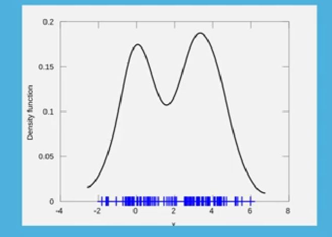
Observations:
- Expected Distribution > peak for Sample 1 at 20, peak for Sample 2 at 40
- ...points in the middle of the distribution, unclear which distribution they belong to
We will use the Gaussian Mixture Model to find out. ChatGPT will be used to explain code lines.
! pip install scikit-learn
# import the gaussian mixture method of scikit learn
from sklearn.mixture import GaussianMixture
# reshape the combined distribution from 1D array to 2D column vector array
# scikit-learn needs 2D data
sample = sample.reshape((len(sample),1)) #parameters are sample length and single value samples
# Create Gaussian Mixture Model with 2 Gaussian components and Random initialization
model = GaussianMixture(n_components=2, init_params='random') # specify that 2 distributions involved and means and covariances are initialized randomly
# generate a fit function for the GMM
model.fit(sample)
GaussianMixture(init_params='random', n_components=2)In a Jupyter environment, please rerun this cell to show the HTML representation or trust the notebook.
On GitHub, the HTML representation is unable to render, please try loading this page with nbviewer.org.
Parameters
| n_components | 2 | |
| covariance_type | 'full' | |
| tol | 0.001 | |
| reg_covar | 1e-06 | |
| max_iter | 100 | |
| n_init | 1 | |
| init_params | 'random' | |
| weights_init | None | |
| means_init | None | |
| precisions_init | None | |
| random_state | None | |
| warm_start | False | |
| verbose | 0 | |
| verbose_interval | 10 |
# Predict the Latent Values from the combined Distribution
y1 = model.predict(sample)
# Check Latent Values for the first and last points
# Easiest way to identify which distribution the points belong to
print(y1[:80]) # check for first 80 points...tend to be with the left most distribution
print(y1[-80:]) # check for last 80 points...tend to be with the right most distribution
[0 0 0 0 0 0 0 0 0 0 0 0 0 0 0 0 0 0 0 0 0 0 0 0 0 0 0 0 0 0 0 0 0 0 0 0 0
 0 0 0 0 0 0 0 0 0 0 0 0 0 0 0 0 0 0 0 0 0 0 0 0 0 0 0 0 0 0 0 0 0 0 0 0 0
 0 0 0 0 0 0]
[1 1 1 1 1 1 1 1 1 1 1 1 1 1 1 1 1 1 1 1 1 1 1 1 1 1 1 1 1 1 1 0 1 1 1 1 1
 1 1 1 1 1 0 1 1 0 1 1 1 1 0 1 1 1 1 1 1 1 1 1 1 0 1 1 1 1 1 0 1 1 1 1 1 1
 1 1 1 1 1 1]
Observations:
I needed ChatGPT to help me to interpret the final output. This is what it said:
- Zeroes represents identification of data points in one cluster
- Ones represents identification of data points in the other cluster
So the output suggests:
- The first 80 points identifies as a mixture between both distributions
- The last 80 points identifies as firmly belonging to the right most distribution
Application of EM Algorithm
- Machine Learning and Computer Vision
- Natural Language Processing
- Quantitative Genetics
- Psychometrics
Advantages and Disadvantages
Advantages
- Guaranteed that likelihood will increase with each iteration
- During implementaton, the e-step and m-step are very easy for many problems
- The solution for m-step often exist in closed form
Disadvantages
- EM algorithm has a very low convergence
- It makes the convergence to the local optima only
- Requires both forward and backward probabilities...a setback when it comes to algorithm in machine learning
Increasing Iterations
I asked ChatGPT how to increase the number of iterations for the GMM. It returned: GMM normally runs 100 EM iterations only
To increase the number of iterations using the Scikit-Learn method, an extra parameter must be added.
I increase the maximum iterations to 500.
# reshape the combined distribution from 1D array to 2D column vector array
# scikit-learn needs 2D data
sample = sample.reshape((len(sample),1)) #parameters are sample length and single value samples
# Create Gaussian Mixture Model with 2 Gaussian components and Random initialization
model = GaussianMixture(n_components=2, init_params='random', max_iter=500) # specify that 2 distributions involved and means and covariances are initialized randomly
# generate a fit function for the GMM
model.fit(sample)
GaussianMixture(init_params='random', max_iter=500, n_components=2)In a Jupyter environment, please rerun this cell to show the HTML representation or trust the notebook.
On GitHub, the HTML representation is unable to render, please try loading this page with nbviewer.org.
Parameters
| n_components | 2 | |
| covariance_type | 'full' | |
| tol | 0.001 | |
| reg_covar | 1e-06 | |
| max_iter | 500 | |
| n_init | 1 | |
| init_params | 'random' | |
| weights_init | None | |
| means_init | None | |
| precisions_init | None | |
| random_state | None | |
| warm_start | False | |
| verbose | 0 | |
| verbose_interval | 10 |
# Predict the Latent Values from the combined Distribution
y1 = model.predict(sample)
# Check Latent Values for the first and last points
# Easiest way to identify which distribution the points belong to
print(y1[:80]) # check for first 80 points...tend to be with the left most distribution
print(y1[-80:]) # check for last 80 points...tend to be with the right most distribution
[0 0 0 0 0 0 0 0 0 0 0 0 0 0 0 0 0 0 0 0 0 0 0 0 0 0 0 0 0 0 0 0 0 0 0 0 0
 0 0 0 0 0 0 0 0 0 0 0 0 0 0 0 0 0 0 0 0 0 0 0 0 0 0 0 0 0 0 0 0 0 0 0 0 0
 0 0 0 0 0 0]
[1 0 0 1 1 0 1 0 1 0 1 1 1 1 1 1 1 1 1 0 1 1 1 1 1 1 1 1 1 1 0 0 0 1 1 1 1
 1 1 1 0 0 0 1 1 0 1 0 1 1 0 1 1 1 1 1 0 0 1 1 1 0 1 0 1 1 1 0 0 0 1 1 1 1
 0 1 1 0 1 1]
Wow!!! A dramatic increase in the result from when it was only 100 iterations!!
Now, the first set of values are identified to clearly belong to the left-most distribution, while the last set of values are identified to clearly belong to the right-most distribution.
Let's see if increasing the iterations to 1000 will make any difference?
# reshape the combined distribution from 1D array to 2D column vector array
# scikit-learn needs 2D data
sample = sample.reshape((len(sample),1)) #parameters are sample length and single value samples
# Create Gaussian Mixture Model with 2 Gaussian components and Random initialization
model = GaussianMixture(n_components=2, init_params='random', max_iter=300) # specify that 2 distributions involved and means and covariances are initialized randomly
# generate a fit function for the GMM
model.fit(sample)
GaussianMixture(init_params='random', max_iter=300, n_components=2)In a Jupyter environment, please rerun this cell to show the HTML representation or trust the notebook.
On GitHub, the HTML representation is unable to render, please try loading this page with nbviewer.org.
Parameters
| n_components | 2 | |
| covariance_type | 'full' | |
| tol | 0.001 | |
| reg_covar | 1e-06 | |
| max_iter | 300 | |
| n_init | 1 | |
| init_params | 'random' | |
| weights_init | None | |
| means_init | None | |
| precisions_init | None | |
| random_state | None | |
| warm_start | False | |
| verbose | 0 | |
| verbose_interval | 10 |
# Predict the Latent Values from the combined Distribution
y1 = model.predict(sample)
# Check Latent Values for the first and last points
# Easiest way to identify which distribution the points belong to
print(y1[:80]) # check for first 80 points...tend to be with the left most distribution
print(y1[-80:]) # check for last 80 points...tend to be with the right most distribution
[0 0 0 0 0 0 0 0 0 1 0 0 0 0 0 0 0 0 0 0 0 0 0 1 0 0 0 1 0 0 1 0 0 1 1 0 0
 1 1 0 0 0 0 0 0 0 0 1 0 0 0 0 0 1 0 0 0 0 0 0 1 0 1 0 0 0 0 1 0 1 1 0 0 0
 0 0 0 0 1 0]
[1 1 1 1 1 1 1 1 1 1 1 1 1 1 1 1 1 1 1 1 1 1 1 1 1 1 1 1 1 1 1 1 1 1 1 1 1
 1 1 1 1 1 1 1 1 1 1 1 1 1 1 1 1 1 1 1 1 1 1 1 1 1 1 1 1 1 1 1 1 1 1 1 1 1
 1 1 1 1 1 1]