Tutorial 1
Gaussian Mixture Models for Clustering from the University of Washington
Notes:
- Mixture of Gaussian
- A gaussian distribution for each variable (cluster) of an analysis (such as image analysis)
- Variables and their (cluster) distributions represents a dimension (brightness, color, etc.) for the image and may have correlation
- Mixing is averaging the (cluster) distributions of the different variable categories
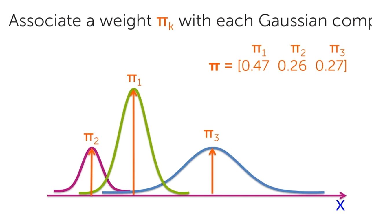
- If one distribution has more data (and influence) than another distribution, percentage Mixture Weights (fraction from 0 to 1) must be multiplied to each distribution to qualify their influence and a Weighted Average distribution calculation performed
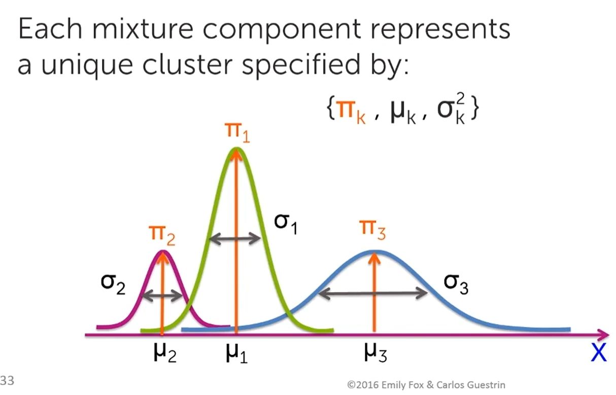
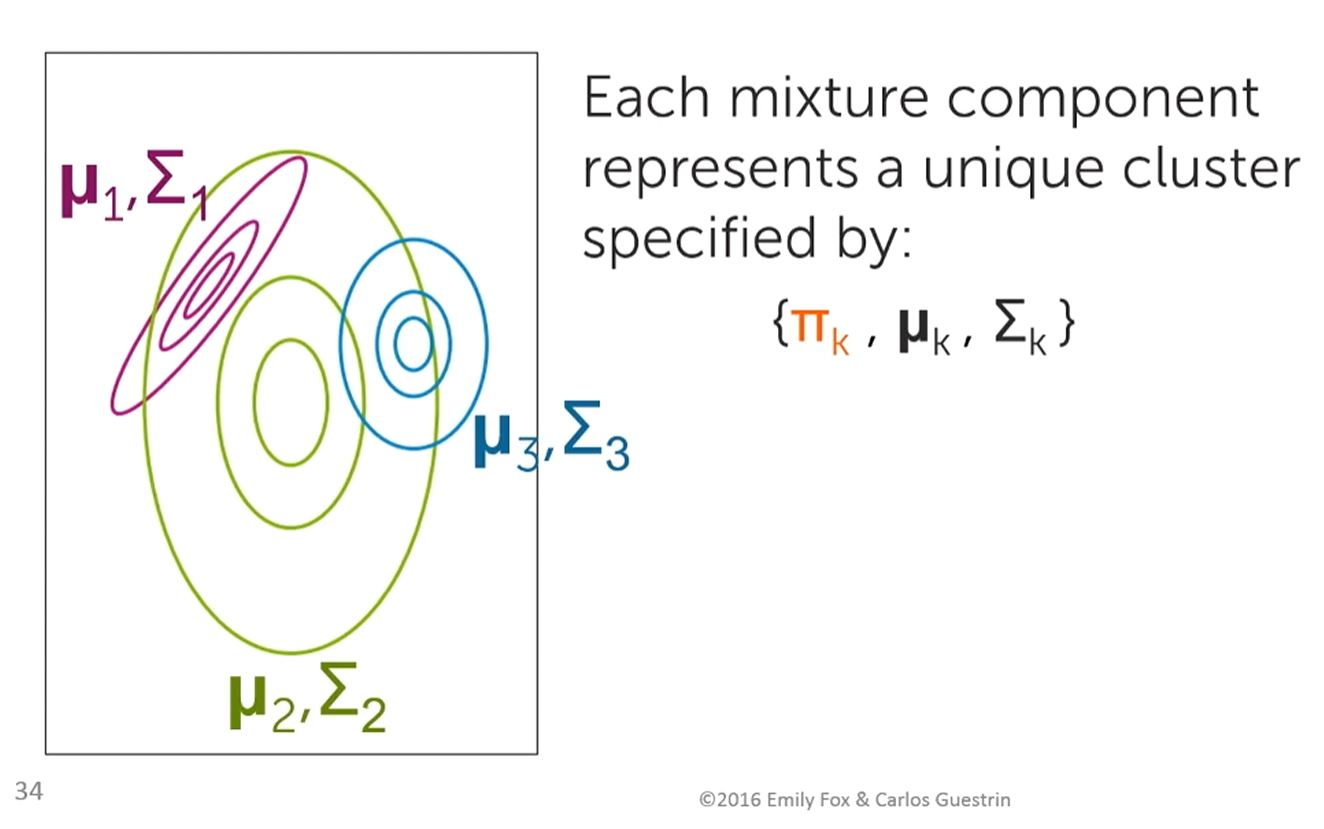
- For each (cluster) distribution, the Mean (mu, location) and Standard Deviation (sigma, spread) values must be specified
- Moving from a 1-dimensional to a 2-dimensional (Contour Plot) representation means that...Covariance (shape & orientation) must also be specified
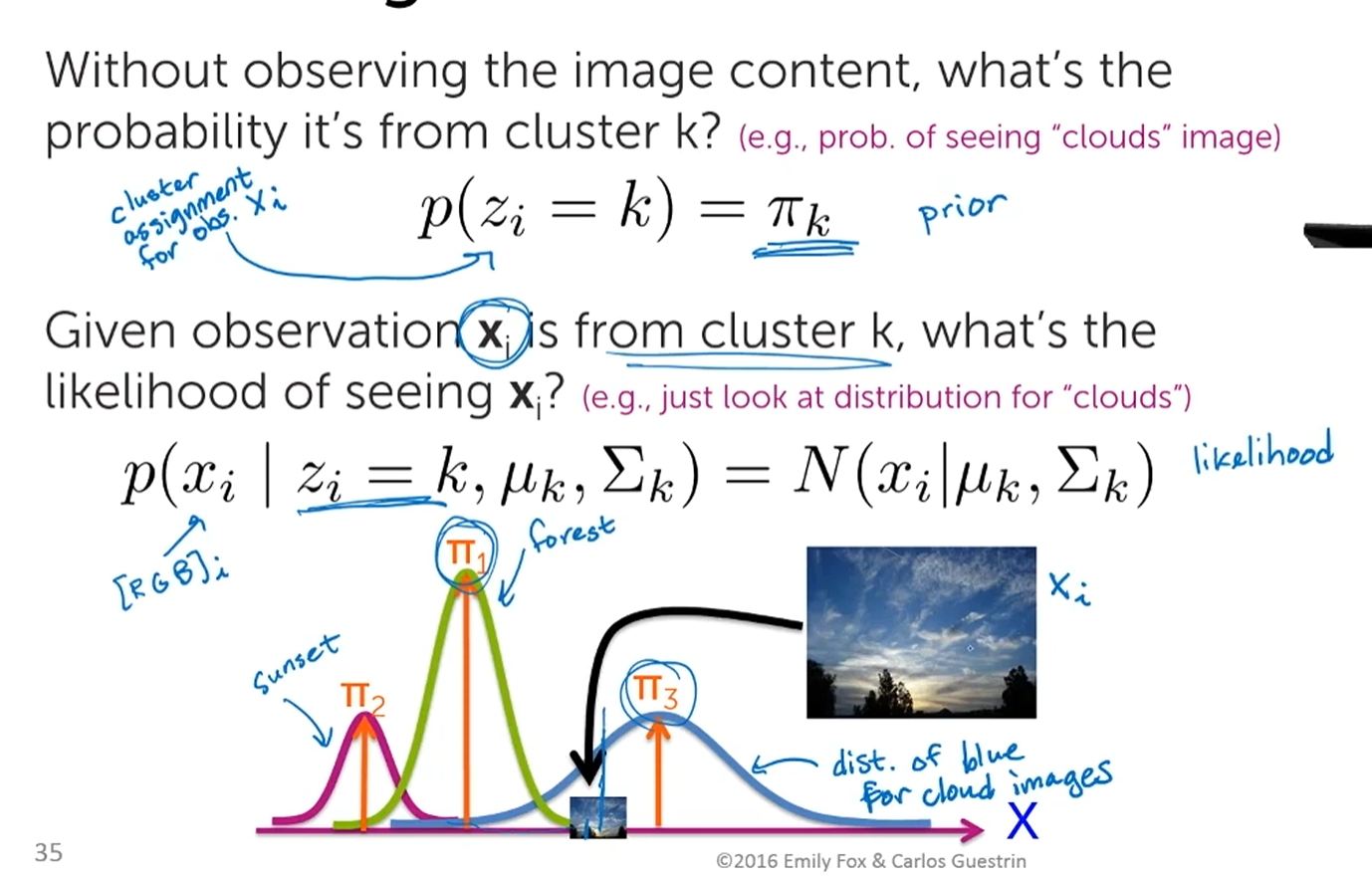
- Cluster Indicator variable 'z', assigns data point observation 'x' to a cluster
Hmmm...after all that, I am still unclear as to what the Gaussian Mixture Model is. What I came away with was...
- that a complex histogram could be made by combining several distributions (cluster of data points) together
- that each cluster is defined by its Mean (mu), Standard Deviation (sigma) and Weight (k)
- that the 2D representation of the distributions is very limiting (a silouette), that the distribution representation in higher dimentions (3 or more) could reveal other relationships between the distributions (3D objects standing apart on a 2D plane...people separated on a square plaza in width and depth)
Next...
Tutorial 2
What are Gaussian Mixture Models? by Six Sigma Pro SMART
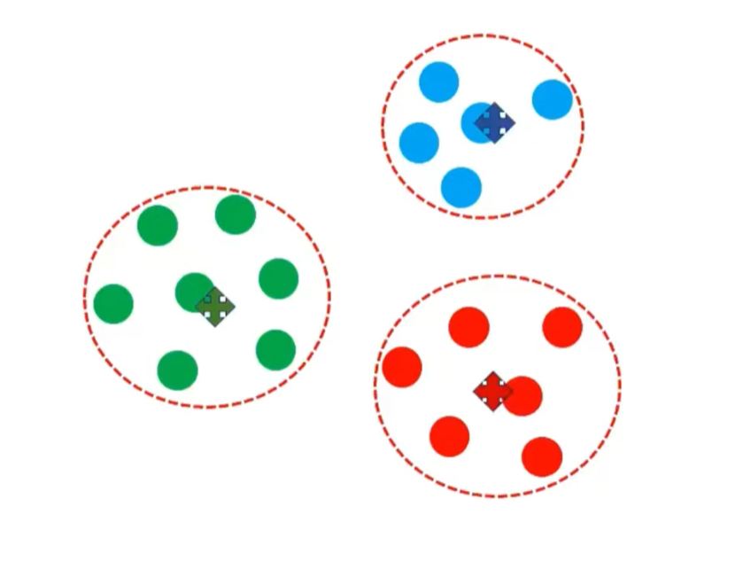
Cleanly separated clusters of similar data, each data point assigned unique cluster label > Hard Clustering
But some data are mixed up...
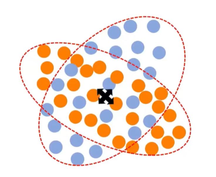
K-means would not work because it is centroid dependent technique and fails when the centroids overlap
Gaussian Mixture Model must be used in this case
If you have a distribution of Real Numbers on a 1D space...'normal' or 'gaussian' distribution algorithm can be applied
...must also decide how many Gaussian Distributions (like how many k-clusters for K-means algorithm) are needed to describe that series of Real Numbers
Procedure:
Randomly initialized the Gaussian
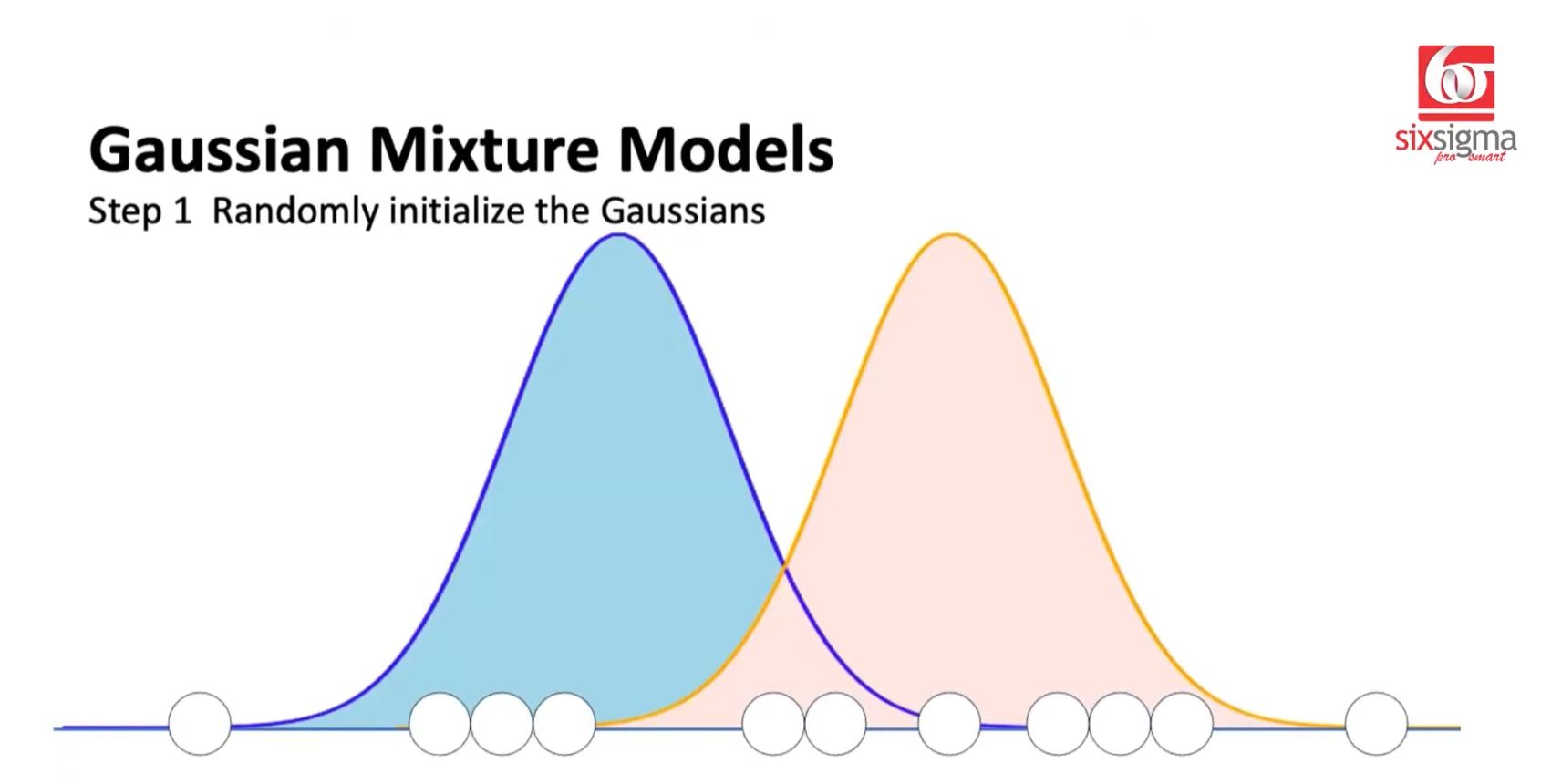
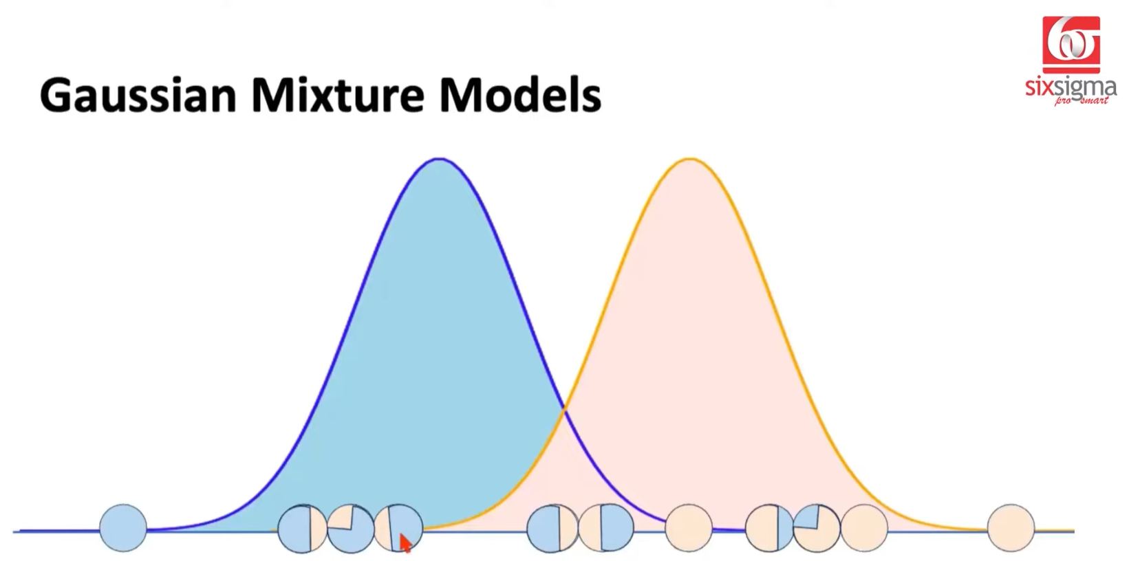
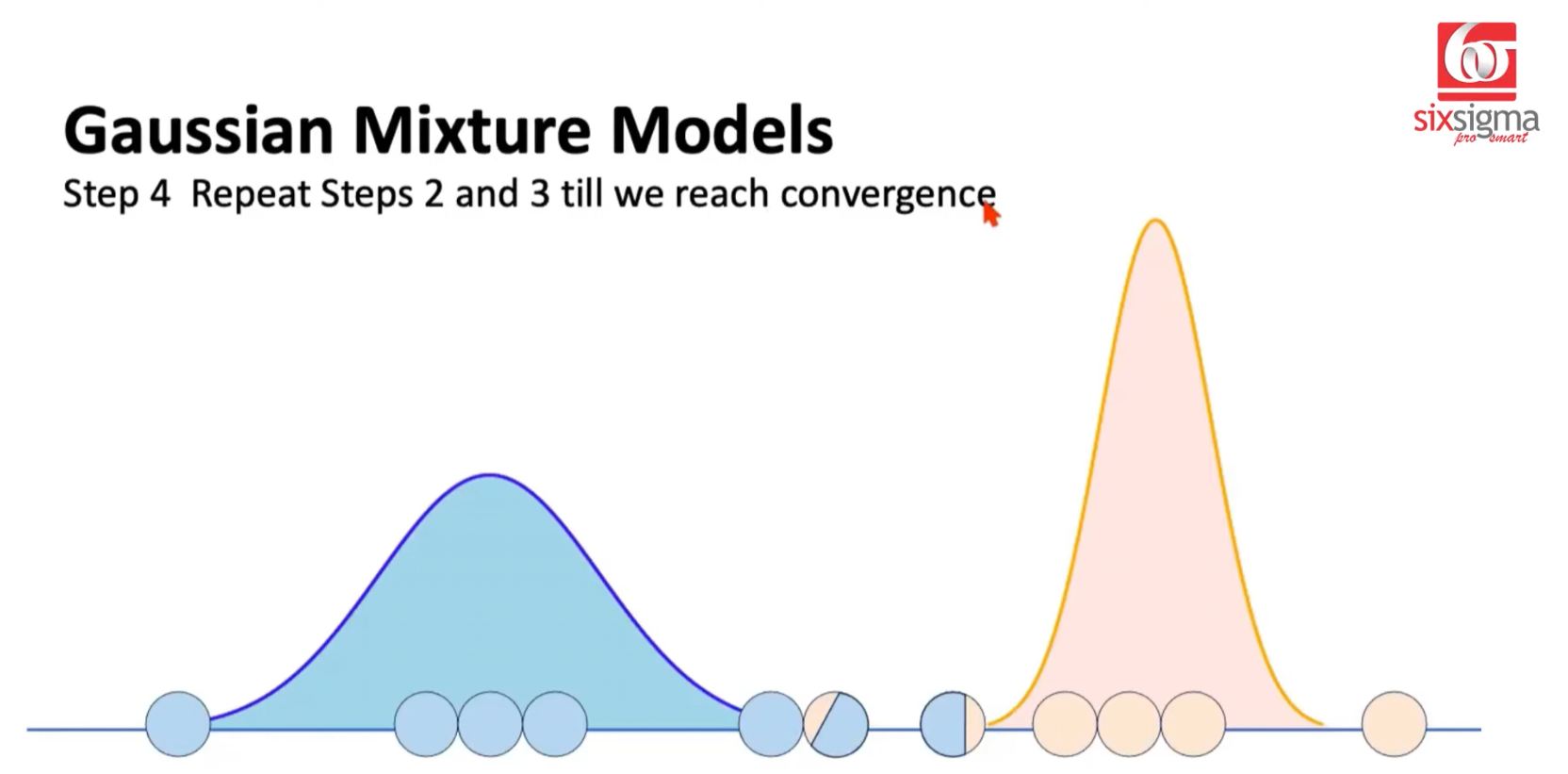
Calculate Responsibility for each Point (Expectation Step) Depending on the point's proximity to one or another Gaussian Distribution, it will exclusively belong to one or be shared by all distributions. When shared, the proximity distance to one distribution versus the other will qualify the fractional influence it has for one distribution vs another.
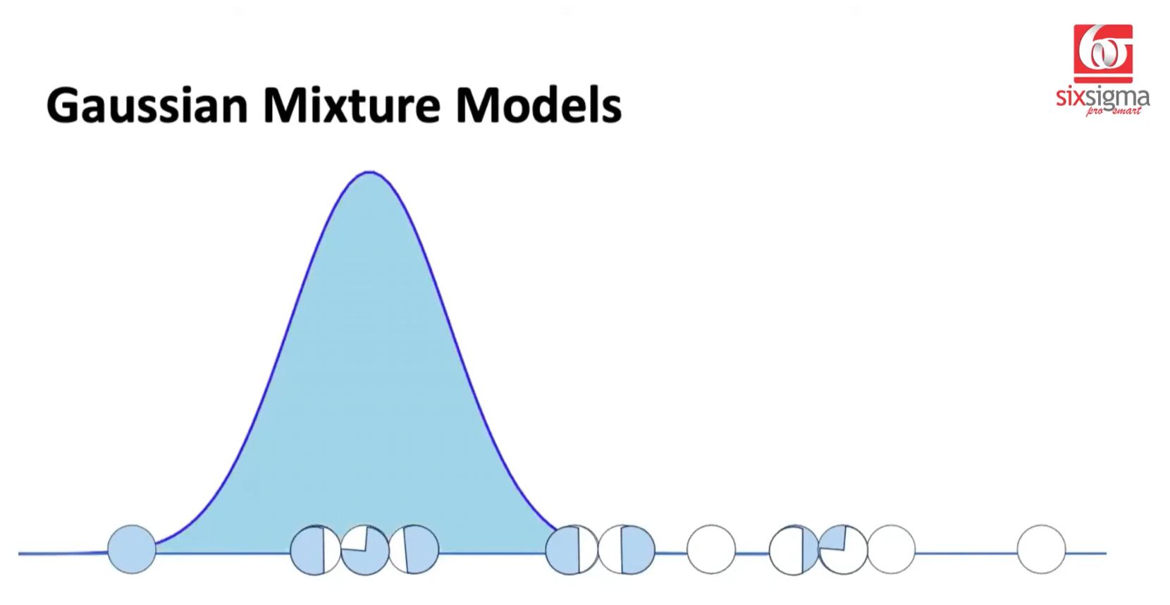
- Reevaluate each Gaussian Distribution based on Responsibility assignments for each point...and recalculate/revise the Normal Distribution (Maximization Step)

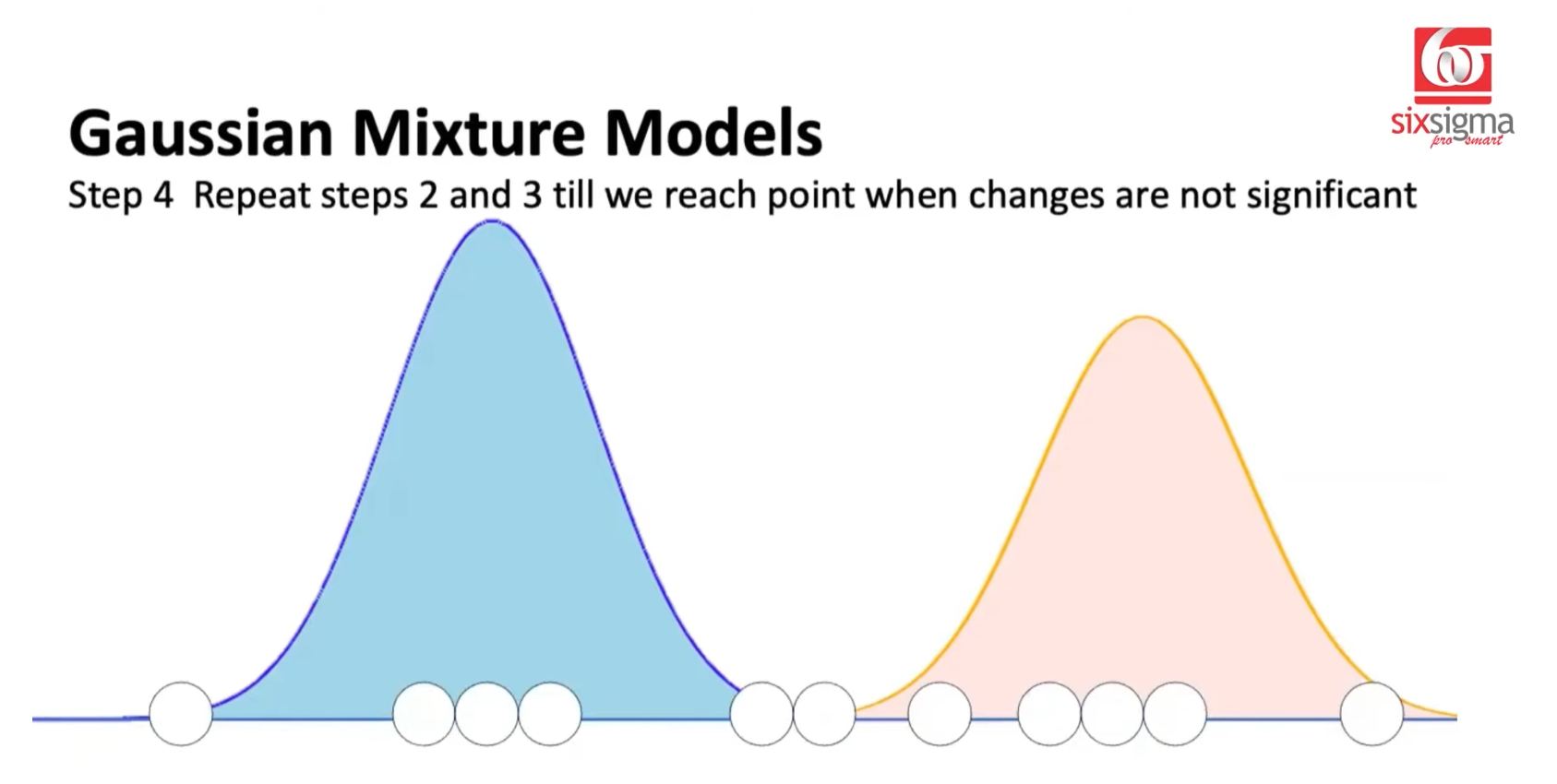
- Repeat Steps 2 and 3 until further changes are insignificant...Convergence reached.
Circular Referencing Calculation
To arrive at the final Gaussian Distribution picture, Responsibities are influence by Gaussians and Gaussian parameters are determined by the responsibilities.
Soft Clustering
Accepting that some data points will influence by more than one Gaussian Distribution...belong to more than one cluster. The K-means technique relies on strict membership to one cluster > Hard Clustering. Gaussian Mixing is a probabilistic model...because it relies on distributions...K-means does not.
Gaussian Mixture is an Expectation Maximization algorithm...because of the iterative way it goes about finding convergence.
Gaussian Mixture in Multi-Dimensional Space
Whereas in 1D space, finding convergence requries the discovery of the correct Mean and Variance...multi-D space will require Mean Vector, Variance-Covariance Matrix...and more complicated mathematics.
Tutorial 3
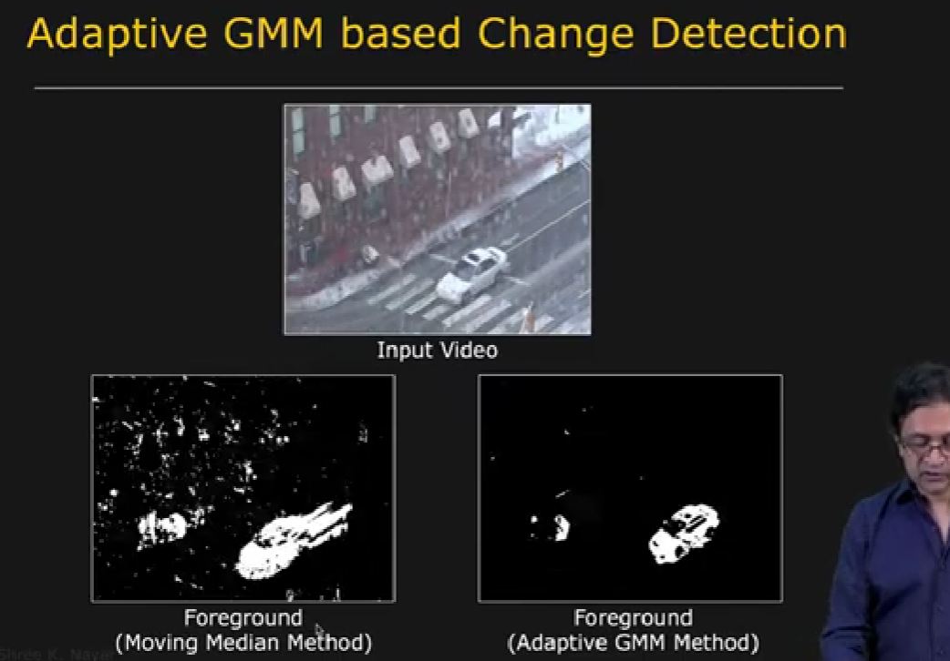
Gaussian Mixture Model|Object Tracking by Dr Shree Nayar, Columbia University
- Change detection algorithms using average or median...but there are limits to these approaches to be resilient to uninteresting changes
- A more sophisticated model for the variation of intensities of colors at each pixel in the image
The objective: counting car from a video image, by isolating it as an 'Object of Interest' from the background image
- Look at the Intensity (brightness) of light for a single pixel...plot as a histogram looking at Intensity over time...with variations due to static scene (road), noise (snow), and occasional moving object (vehicles...a rare event).
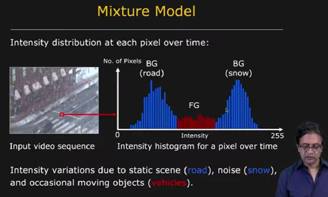
- The image shows 2 primary distributions in light intensity...road and snow
- ...and a 3rd distribution, representing the occasional passing of a car through the image
- Intuition: "pixels are background most of the time"
- Approach: Classify pixels as belonging to the background or the foreground (car)
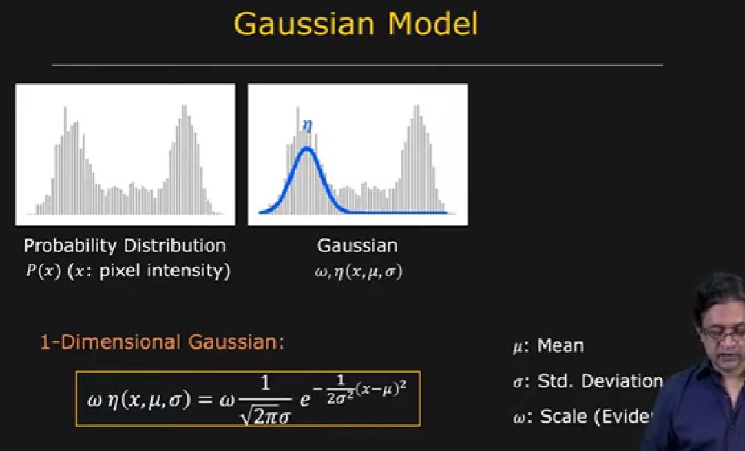
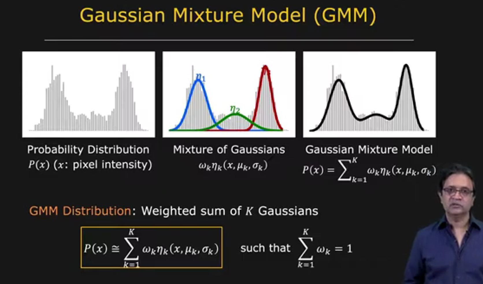
Define a 1D Gaussian distribution for aspects of the Histogram with 3 key parameters, Mean/Location (mu), Standard Deviation/Width (sigma), and Scale/Evidence (omega)
View the Histogram as a collection of Gaussians.
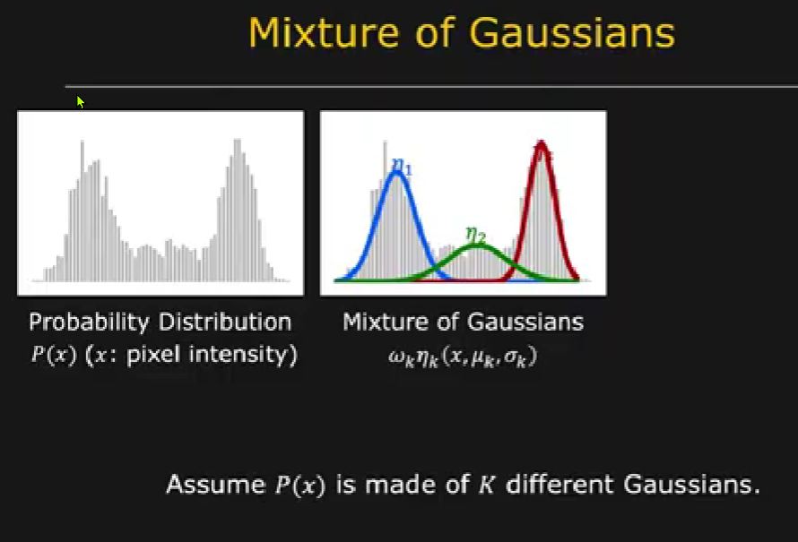
Find the parameters of these Gaussians then generate a Mixture of Gaussians (sum) Fit Function for the Histogram.
GMM Distribution = Weighted sum of K Gaussians
- sum of omega must equal to 1
Can be taken to higher dimensions. For the image example, not just look at Brightness (Intensity) but also 3 channels of color (red, green, blue).
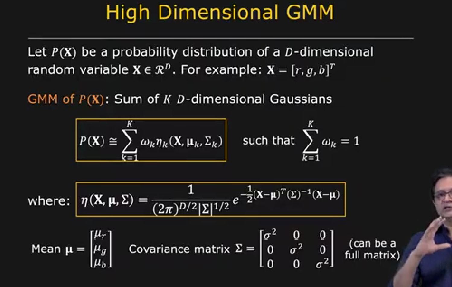
Still sum of gaussian distributions, but for high dimensional mixtures:
- Means becomes a matrix of Mean Vectors
- Standard Deviation becomes a matrix of Covariances
A GMM can be estimated from any Probability distribution, regardless of dimensionality.
Decide what k is, how many Gaussians to use for the mix and fit. If k is large...the fit can become unstable. If k is too small...the fit will lack flexibility and be inaccurate.
Practical Example
Given: A GMM for intensity/color variation at a pixel over time
Classify: Individual Gaussians as either foreground/background
Intuition: Pixels are background most of the time. Gaussians with large supporting evidence (scale) and small sigma (width)...is background.
Develop the Algorithm (simplified Stauffer algorithm)
For each pixel:
Compute pixel color histogram H using first N frames.
Normalize histogram (make sure is a distribution)
Model Normalized Histogram as mixture of K (3 to 5) Gaussians.
(Classifying) For each subsequent frame:
a. The pixel value X belongs to Gaussian k in GMM for which X to meanK is minimum, and X to meanK Mis less than 2.5sigmaK. Find which gaussian distribution's mean value the pixel value is closest to and also if the distance is below a certain threshold value.
b. If omega/sigma is large, then classify pixel as background. Else classify as foreground.
c. Update the histogram using new pixel intensity.
d. If Normalized Histogram and New Histogram differ a lot...then replace the old histogram with the new histogram...and refit the GMM.
Region of Interest identified:
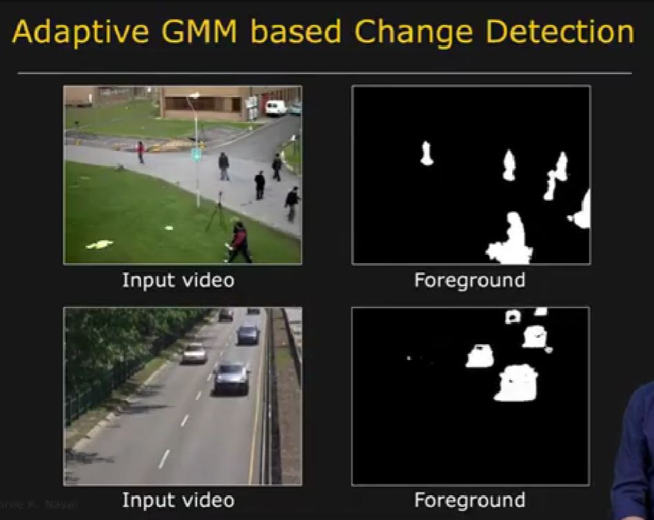
...can be used for further processing.