FAB Futures - Data Science

Home About

Research > Machine Learning

Deconstructing Neil's Machine Learning Code

Oh man, the last Data Science with Neil was a tough one. Not only was it highly technical with lots of new, mysterious jargon...but I was particularly sleepy at 11:00PM when the class took place. My murky brain had only 3 takeaways:

• Machine Learning
• JAX
• Character Recognition

While I intend on watching the recording of the lecture one more time, I thought it would be worthwhile to spend some time to deconstruct Neil's Machine Learning code line-by-line...with the help of my personal tutor, ChatGPT.

This is Neil's full code...

#!/usr/bin/env python3
"""
Minimal JAX MNIST trainer (JAX + matplotlib + Python stdlib only).
Downloads MNIST from https://raw.githubusercontent.com/fgnt/mnist/master
"""

import gzip
import struct
import urllib.request

import jax
import jax.numpy as jnp
from jax import random, jit, grad
import matplotlib.pyplot as plt


# --------------------- Download + parse MNIST (IDX format) ---------------------
SERVER = "https://raw.githubusercontent.com/fgnt/mnist/master"
FILES = {
    "train_images": "train-images-idx3-ubyte.gz",
    "train_labels": "train-labels-idx1-ubyte.gz",
    "test_images":  "t10k-images-idx3-ubyte.gz",
    "test_labels":  "t10k-labels-idx1-ubyte.gz",
}

def fetch_bytes(path):
    with urllib.request.urlopen(f"{SERVER}/{path}") as r:
        return r.read()

def parse_idx_images(gz_bytes):
    data = gzip.decompress(gz_bytes)
    magic, n, rows, cols = struct.unpack(">IIII", data[:16])
    assert magic == 2051, f"Bad magic for images: {magic}"
    # Read the remaining bytes as uint8, then normalize to [0,1] and flatten.
    arr = jnp.frombuffer(data, dtype=jnp.uint8, offset=16)
    arr = arr.reshape((n, rows * cols)).astype(jnp.float32) / 255.0
    return arr

def parse_idx_labels(gz_bytes):
    data = gzip.decompress(gz_bytes)
    magic, n = struct.unpack(">II", data[:8])
    assert magic == 2049, f"Bad magic for labels: {magic}"
    lab = jnp.frombuffer(data, dtype=jnp.uint8, offset=8).astype(jnp.int32)
    return lab

def load_mnist():
    trX = parse_idx_images(fetch_bytes(FILES["train_images"]))
    trY = parse_idx_labels(fetch_bytes(FILES["train_labels"]))
    teX = parse_idx_images(fetch_bytes(FILES["test_images"]))
    teY = parse_idx_labels(fetch_bytes(FILES["test_labels"]))
    return trX, trY, teX, teY


# ------------------------------- Tiny JAX MLP ---------------------------------
def init_params(key, d_in=784, d_hidden=128, d_out=10):
    k1, k2 = random.split(key)
    W1 = random.normal(k1, (d_in, d_hidden)) * jnp.sqrt(2.0 / d_in)
    b1 = jnp.zeros((d_hidden,))
    W2 = random.normal(k2, (d_hidden, d_out)) * jnp.sqrt(2.0 / d_hidden)
    b2 = jnp.zeros((d_out,))
    return {"W1": W1, "b1": b1, "W2": W2, "b2": b2}

def forward(params, x):
    h = jax.nn.relu(x @ params["W1"] + params["b1"])
    return h @ params["W2"] + params["b2"]  # logits

@jit
def predict(params, x):
    return jnp.argmax(forward(params, x), axis=-1)

@jit
def cross_entropy_loss(params, x, y):
    logits = forward(params, x)
    y_one = jax.nn.one_hot(y, num_classes=logits.shape[-1])
    logp = jax.nn.log_softmax(logits)
    return -jnp.mean(jnp.sum(y_one * logp, axis=-1))

@jit
def accuracy(params, x, y):
    return jnp.mean(predict(params, x) == y)

@jit
def sgd_step(params, x, y, lr):
    grads = grad(cross_entropy_loss)(params, x, y)
    return {k: params[k] - lr * grads[k] for k in params}


# ------------------------------ Training helpers ------------------------------
def train(train_X, train_y, test_X, test_y, epochs=5, batch_size=128, lr=0.1, seed=0):
    key = random.PRNGKey(seed)
    params = init_params(key)
    n = train_X.shape[0]

    for epoch in range(1, epochs + 1):
        key, sk = random.split(key)
        perm = random.permutation(sk, n)
        for i in range(0, n, batch_size):
            idx = perm[i:i + batch_size]
            params = sgd_step(params, train_X[idx], train_y[idx], lr)

        # quick epoch metrics on small subsets (for speed)
        tr_loss = cross_entropy_loss(params, train_X[:2000], train_y[:2000])
        tr_acc  = accuracy(params, train_X[:2000], train_y[:2000])
        te_acc  = accuracy(params, test_X, test_y)
        print(f"Epoch {epoch:2d} | loss {float(tr_loss):.4f} | "
              f"train_acc {float(tr_acc):.4f} | test_acc {float(te_acc):.4f}")
    return params

def show_samples(X, y, params=None, ncols=8):
    fig, axes = plt.subplots(1, ncols, figsize=(ncols * 1.4, 1.8))
    for i in range(ncols):
        img = X[i].reshape(28, 28)
        axes[i].imshow(img, cmap="gray", interpolation="nearest")
        title = f"label={int(y[i])}"
        if params is not None:
            pred = int(predict(params, X[i:i+1])[0])
            title += f"\npred={pred}"
        axes[i].set_title(title, fontsize=8)
        axes[i].axis("off")
    plt.tight_layout()
    plt.show()


# ------------------------------------ Main ------------------------------------
def main():
    print("Downloading + loading MNIST...")
    train_X, train_y, test_X, test_y = load_mnist()
    print("Train:", train_X.shape, train_y.shape, "| Test:", test_X.shape, test_y.shape)

    print("Showing a few training samples (ground-truth labels)...")
    show_samples(train_X, train_y, params=None)

    print("Training...")
    params = train(train_X, train_y, test_X, test_y, epochs=5, batch_size=128, lr=0.1)

    print("Showing samples with model predictions (fits)...")
    show_samples(train_X, train_y, params=params)

main()

I asked for an explanation from ChatGPT and this is how it described the above code...

"It downloads MNIST, builds a tiny neural network in JAX, trains it, and shows sample digits + predictions."

OK, some jargon to be defined:

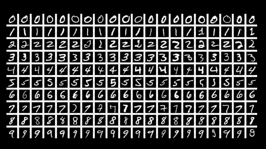
MINST = "a database of handwritten digits that is commonly used for training various image processing systems" wikipedia

- Downloadable digital images of numerical and alphabetical characters used for Machine Learning model training  

Tiny Neural Network = "...is an efficient and easy-to-use deep learning model compression framework." alibaba github

- A lightweight, basic Neural Network model with features like "neural architecture search, pruning, quantization, model conversion, and etc."  
- More accessible and easier to use that bigger, more complicated Neural Network models  

JAX = "JAX is a Python library for accelerator-oriented array computation and program transformation, designed for high-performance numerical computing and large-scale machine learning." JAX Documentation

- From my understanding, JAX is essentially a version of NUMPY that is able to make calculations much more efficiently and speedily.   

Code Deconstruction > Imports & Descriptions

In ChatGPT, I prompted "explain this code" and pasted Neil's full code. The following is ChatGPT's breakdown and explanation of the code.

Neil describes the program as a...*"Minimal JAX MNIST trainer (JAX + matplotlib + Python stdlib only)." and that we should go download the MNIST dataset from the following website

The topmost section of code imports all the needed libraries for the program.

import gzip
import struct
import urllib.request

import jax
import jax.numpy as jnp
from jax import random, jit, grad
import matplotlib.pyplot as plt

gzip = a data compression/decompression utility. W3schools.com provides the following definitions..."The gzip module provides a simple interface for compressing and decompressing data using the gzip format."

struct = from doc.python.org, this utility "interprets bytes as packed binary data"

urllib.request = "is a package that collects several modules for working with URLs" according to doc.python.org

jax.numpy = is an API that translates jax functionality to numpy, because "While JAX tries to follow the NumPy API as closely as possible, sometimes JAX cannot follow NumPy exactly." according to JAX documentation

random = is a JAX "package (that) provides a number of routines for deterministic generation of sequences of pseudorandom numbers." according to JAX documentation

jit = "Just-in-Time" compilation for Python, " take a standard Python function operating on JAX arrays and convert it into a highly optimized, fused sequence of operations specific to your hardware (CPU, GPU, or TPU" according to APXML. Speeds up code runtime.

grad = "is a key feature of JAX that provides automatic differentiation, allowing you to compute gradients of functions efficiently." according to Medium.com

matplotlib.pyplot = is used for making visualizations such as data plots...and in this case images of digits.

the next section of code, downloads the MNIST character image files:

The location of the files... Assigns the MNIST file location name to the variable "Server".

SERVER = "https://raw.githubusercontent.com/fgnt/mnist/master"
FILES = {
    "train_images": "train-images-idx3-ubyte.gz",
    "train_labels": "train-labels-idx1-ubyte.gz",
    "test_images":  "t10k-images-idx3-ubyte.gz",
    "test_labels":  "t10k-labels-idx1-ubyte.gz",
}

Downloads the raw bytes..."

def fetch_bytes(path):
    with urllib.request.urlopen(f"{SERVER}/{path}") as r:
        return r.read()

ChatGPT says the next section Parses the image files (IDX format), which it further explains to mean..."reading and interpreting a special binary file format called IDX (not PNG or JPEG) used by MNIST to store its images and labelss...and converts it into usable image arrays"

IDX contains:

• a Header, "magic number", number of items, rows, columns

• RAW Bytes of pixel data or label data...uncompressed, no metadata or image encoding

• Parsing means:

• read the file bytes

• check the header (how many images contained)

• extract pixel data

• reshape pixels into 28x28 images

• convert them into model-usable arrays

def parse_idx_images(gz_bytes):
    data = gzip.decompress(gz_bytes) #unzip
    magic, n, rows, cols = struct.unpack(">IIII", data[:16]) #reads first 16-bytes as 4 unsigned integers
    assert magic == 2051, f"Bad magic for images: {magic}" #check that it is an image file  
    arr = jnp.frombuffer(data, dtype=jnp.uint8, offset=16) #interprets the remaining bytes as unsigned 8-bit intergers (pixel values 0 to 255)
    arr = arr.reshape((n, rows * cols)).astype(jnp.float32) / 255.0 #each image converted to a 1D vector with length 28x28=784...converts to float 32 and divide by 255 to arrive at either 0 or 1 (normalizing)
    return arr

The next section Parses the Label File

Similar to the previous procedure for images, this time for just the "Labels".

def parse_idx_labels(gz_bytes):
    data = gzip.decompress(gz_bytes) #decompresses
    magic, n = struct.unpack(">II", data[:8]) #reads 8-bytes header
    assert magic == 2049, f"Bad magic for labels: {magic}" #check that it is a header file
    lab = jnp.frombuffer(data, dtype=jnp.uint8, offset=8).astype(jnp.int32) #interprets remaining bytes as integers from 0 to 9 (digit labels) 
    return lab

The next section Loads all MNIST Splits. What I understand this to be is that the parsed image and label data are downloaded then separated into 4 distinct sets and assigned to a unique variable.

The 4 sets include:

• training images > trX
• training labels > trY
• testing images > teX
• testing labels > teY

def load_mnist():
    trX = parse_idx_images(fetch_bytes(FILES["train_images"]))
    trY = parse_idx_labels(fetch_bytes(FILES["train_labels"]))
    teX = parse_idx_images(fetch_bytes(FILES["test_images"]))
    teY = parse_idx_labels(fetch_bytes(FILES["test_labels"]))
    return trX, trY, teX, teY

With all the libraries imported and image data and labels downloaded, now the code moves into the Neural Network and Machine Learning Model building procedure.

Defining the Tiny Neural Network (MLP).

MLP = not "My Little Pony" (what the Google search returned) but rather a Multilayer Perceptron (according to ChatGPT)..."the simples type of Neural Network made of fully connected (dense) layers"

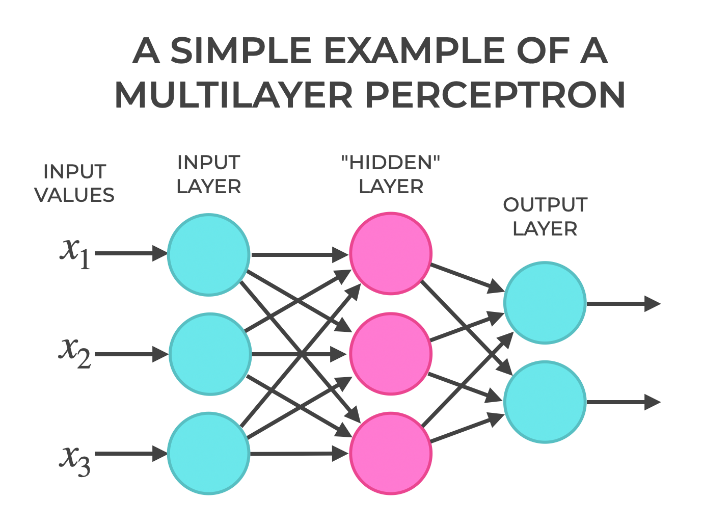
According to Wikipedia, an MLP is a "feedforward Neural Network" (an artificial neural network in which information flows in a single direction) consisting of fully connected neurons with nonlinear "activation functions" (a node function that calculates the output of the node based on its individual inputs and their weights), organized in layers, notable for being able to distinguish data that is not linearly separable."

"Neural Networks are trained using "backpropagation"(a loss-function respective to weights of the network, gradient computation method)" where gradient computation is done one layer at a time, interating backward from the last layer to avoid redundant calculations..."*

According to geeksforgeeks.com...an MLP "is called multi-layer because it contains an input layer, one or more hidden layers and an output layer. The purpose of an MLP is to model complex relationships between inputs and outputs."

MLPs are Simple

• only matrix multiplication + activation functions
• general-purpose > can learn many types of functions (classification, regression)
• is "dense" > every input influences every Neuron

The Key Components of an MLP are:

Input Layer... the first layer responsible for receiving raw input values Hidden Layer...can be one or more intermediate layers between input and output, performing most of the computation required applying weights and biases to the input data, followed by an activation function to introduce non-linearity. geeksforgeeks.org
Output Layer..."the final layer, produces the output predictions. The number of neurons in the layer corresponds to the number of classification categories to be predicted. The "Activation Function" used in the output layer depends on the type of problem: Softmax for multi=class classification, Sigmoid for Binary Classification, or linear for Regression".

from geeksforgeeks.org

MLP is good for MNIST

• MNIST images are small (28x28)
• A simple MLP can reach 97% accuracy with minimal code
• It's fast to train More advanced models like CNNs (Convolutional Neural Networks) perform better, but an MLP is the easiest starting point. (ChatGPT)

Initialize Neuro Network Parameters

• w = weights, how strongly each input influences each subsequent neuron
• b = biases, vector added to each layer's output before activation, allow neurons to 'shift' their activation threshold, allows for 'expression'

def init_params(key, d_in=784, d_hidden=128, d_out=10): #784 datapoints, 128 hidden layers, 10 output layers
    k1, k2 = random.split(key) # split the randomly generated PRNG key into 2
    W1 = random.normal(k1, (d_in, d_hidden)) * jnp.sqrt(2.0 / d_in) #weight matrix input > hidden...random normal values scaled by sqrt(2/fan_in)
    b1 = jnp.zeros((d_hidden,)) 
    W2 = random.normal(k2, (d_hidden, d_out)) * jnp.sqrt(2.0 / d_hidden) #weight matrix hidden > output...random normal values scaled by sqrt(2/fan_in)
    b1 = jnp.zeros((d_hidden,)) #bias for hidden neuron...init = 0
    b2 = jnp.zeros((d_out,)) #bias for output class...init = 0
    return {"W1": W1, "b1": b1, "W2": W2, "b2": b2}

Forward Pass

According to ChatGPT...

• x is a batch of INPUTs '
• Apply ReLU to the First Layer
• Apply generates Logits

ReLU = Rectified Linear Unit

• A common Activation Functions used in Neural Networks, including MLPs
• The Formula: ReLU(x) - max(0,x)
  • If INPUT is Positive, keep it
  • if INPUT is Negative, output 0
• ReLU helps Neural Networks learn faster...avoids the 'slow saturating' behavior of older activations (sigmoid, tanh)
• Other activations (sigmoid or tanh) squashes values, killing gradients
• Compares to 0 > no exponentials, no trigonometry
• ReLU 'rectifies' data (removes non positivie values)

Logit = raw output score of a Neural Netowrk, before it is turned into a probability (ChatGPT)

• The number produced by the Neural Network before Softmax
• A real number (positive, negative, or zero) representing how strongly the model believes n input belongs to a class
• While not probabilities, the class with the largest logit is usually the prediction

ex: For MLP outputs for digits 0-9 , if logits as follows... [-2.1, 0.3, 1.7, 5.2, -0.3, 0.0. 0.4. -3.0, 2.8, 1.2]

...5.2 is the highest value and is in the 4th index position associated with the number '3'.

Softmax

• Softmax turns logits into probabilities
• The Formula: probability = logit/sum of logits

def forward(params, x):
    h = jax.nn.relu(x @ params["W1"] + params["b1"]) #apply ReLU at first layer, x is input size (784)
    return h @ params["W2"] + params["b2"]  # gives logits (raw scores, not probabilities), output size = output categories

Predictions

ChatGPT explains...

• jit tells JAX to compile the function for speed
• runs the 'forward' function then picks the class with the largest logit for each sample

@jit #compile for speed
def predict(params, x):
    return jnp.argmax(forward(params, x), axis=-1) #runs forward & picks the class with the largest logit

Loss Function (Cross Entropy)

• run the 'forward' function to get logit values, assign values to the variable 'logits'
• 'one hot' encode labels > assign the number 1 to the index position of generated logits, assign to the variable 'y_one'
• generate softmax probabilities for each logit with log_softmax, assign to the variable 'logp'
• returns the calculated mean value

@jit
def cross_entropy_loss(params, x, y):
    logits = forward(params, x)
    y_one = jax.nn.one_hot(y, num_classes=logits.shape[-1])
    logp = jax.nn.log_softmax(logits)
    return -jnp.mean(jnp.sum(y_one * logp, axis=-1))

Accuracy

ChatGPT explains...

• how many predictions are correct, then returns the fraction that are correct
• gets the model generated predictions and compares to true labels for each digit
• on a boolean array gives the fraction of correct predictions (if the prediction matches the correct digit, assign 'true')

The Accuracy Function checks every prediction...correct ones count as 1, wrong ones count as 0, averages them, and provides the accuracy score

@jit
def accuracy(params, x, y):
    return jnp.mean(predict(params, x) == y)

One SGD Update Step

ChatGPT explains...

This function does one training step of Stochastic Gradient Descent (SGD)

1. Compute how much the loss changes with respect to each parameter (the gradient)
2. Move each parameter a tiny bit in the direction that reduces the loss

grad(cross_entropy_loss

• a function that computes the gradient of the loss with respect to the parameters...the derivative (slope) of the loss with respect to each entry in W1, b1, W2, b2

Gradient Descent:

1. Take the current parameter (params[k])
2. Take its gradient (grads[k])
3. Multiply the gradient by the Learning Rate (lr)
   • controls the step size
4. Subtract it from the current parameter
   • to minimize the loss
5. Store the result in a new dictionary (new_params)

...move each parameter a little bit opposite the gradient to reduce the loss.

SGD

Gradient Descent is a methond to train a Neural Network by adjusting its parameters (weights and biases) so the loss goes down. Starting from a point on the gradient and knowing the slope, adjust the point position slightly, down the slope...to reach the lowest point (minimum loss).

A normal gradient descent (Batch Gradient Descent), which compute the loss using all data at once, is slow and uses too much memory.

Stochastic Gradient Descent (SGD) uses a small random subset to estimate the slope.

1. Pick a random batch of data (Stochastic = random)
2. Compute the Loss for that batch
3. Compute the Gradient, tells you which direction increases loss the most
4. Update parameters the opposite way (reduces the loss)
5. Grab another random batch > repeat (and the model learns)

@jit
def sgd_step(params, x, y, lr):
    grads = grad(cross_entropy_loss)(params, x, y)
    return {k: params[k] - lr * grads[k] for k in params} #adjust each parameter in the direction that reduces the loss 

Training Loop

ChatGPT explains...

• Create a random key from the seed
• Initializes parameters
• n = the number of training examples

def train(train_X, train_y, test_X, test_y, epochs=5, batch_size=128, lr=0.1, seed=0):
    key = random.PRNGKey(seed)
    params = init_params(key)
    n = train_X.shape[0]

Epoch Loop

• For each epoch, split the key again
• Give a random permutation of indices (shuffles the dataset)

    for epoch in range(1, epochs + 1):
        key, sk = random.split(key)
        perm = random.permutation(sk, n)

Mini-Batch Loop

• walks through the training data in chunks
• 'idx' selects a slice of shuffled indices
• takes the mini-batch and performs an SGD Step to update the parameters

        for i in range(0, n, batch_size):
            idx = perm[i:i + batch_size]
            params = sgd_step(params, train_X[idx], train_y[idx], lr)

Compute Metrics for Each Epoch

• Evalutates on all test data, one batch at a time
• Returns the trained parameters at the end

        # quick epoch metrics on small subsets (for speed)
        tr_loss = cross_entropy_loss(params, train_X[:2000], train_y[:2000])
        tr_acc  = accuracy(params, train_X[:2000], train_y[:2000])
        te_acc  = accuracy(params, test_X, test_y)
        print(f"Epoch {epoch:2d} | loss {float(tr_loss):.4f} | "
              f"train_acc {float(tr_acc):.4f} | test_acc {float(te_acc):.4f}")
    return params

Visualizing Samples

def show_samples(X, y, params=None, ncols=8):
    fig, axes = plt.subplots(1, ncols, figsize=(ncols * 1.4, 1.8))
    for i in range(ncols):
        img = X[i].reshape(28, 28)
        axes[i].imshow(img, cmap="gray", interpolation="nearest")
        title = f"label={int(y[i])}"
        if params is not None:
            pred = int(predict(params, X[i:i+1])[0])
            title += f"\npred={pred}"
        axes[i].set_title(title, fontsize=8)
        axes[i].axis("off")
    plt.tight_layout()
    plt.show()

• show a row of images 28px by 28px in size