Yosuke Tsuchiya - Fab Futures - Data Science

Home About

Week 02-02: Machine Learning

Assignment: Fit a machine learning model to your data

Plan

Using my Prusa Core One Printer log, it is difficult part for me to apply machine learnig to them. I want to predict something from the log... So, I decided to predict the following values:

• to predict the total move of extruder position (how much extruder moved = filament used)

Also, I tried to add more variables from calculation of log data.

Please also see my previous documents:

• Get Prusa 3D Printer Status with Python (rev.1)
• Week01-02 assignment (visualizing 3D print log)

Preparation

Function to parse printing log data

First, define functions to read printer logs.

import pandas as pd
import numpy as np
import matplotlib.pyplot as plt
from datetime import datetime,timedelta,timezone

Here is the function to read the temperture log and return them as Data Frame. There are nothing to changed from the last class assignment.

def get_printer_temp_data(path):

    with open(path,"r") as tf:
        temp_data = tf.readlines()
    
    resjson = []
    last_time = ''
    total_printing_time = 0.0
    start_time = 0.0
    
    for item in temp_data:

        tempdata = item.split(' ')
        
        addjson = {}
        logtime = tempdata[0]

        t = logtime.split('.')
        tp = datetime.strptime(t[0],'%Y/%m/%d-%H:%M:%S')

        #if last_time != "":
        #    if tp == datetime.strptime(last_time,'%Y/%m/%d-%H:%M:%S'):
        #        continue
        logtime = t[0]
        addjson['logtime'] = logtime.replace('-',' ')
        last_time = logtime
        
        nozzle_temps = str(tempdata[1]).replace('T:','')
        nozzle_temp_current,nozzle_temp_setting = nozzle_temps.split('/')
        addjson['hotend_temp_current'] = float(nozzle_temp_current)
        addjson['hotend_temp_setting'] = float(nozzle_temp_setting)
        
        bed_temps = str(tempdata[2]).replace('B:','')
        bed_temp_current,bed_temp_setting = bed_temps.split('/')
        addjson['bed_temp_current'] = float(bed_temp_current)
        addjson['bed_temp_setting'] = float(bed_temp_setting)
    
        heatbreak_temps = str(tempdata[3]).replace('X:','')
        heatbreak_temp_current,heatbreak_temp_setting = heatbreak_temps.split('/')
        addjson['heatbreak_temp_current'] = float(heatbreak_temp_current)
        addjson['heatbreak_temp_setting'] = float(heatbreak_temp_setting)
    
        hotend_power = str(tempdata[5])
        hotend_power = hotend_power.replace('@:','')
        #0-255 (mapping 0.0-100.0)
        hotend_power = (float(hotend_power) / 255) * 100
        addjson['hotend_power'] = hotend_power
        
        bed_heater_power = str(tempdata[6])
        bed_heater_power = bed_heater_power.replace('B@:','')
        bed_heater_power = (float(bed_heater_power) / 255) * 100
        addjson['bed_heater_power'] = bed_heater_power

        hotend_fan_power = str(tempdata[8])
        hotend_fan_power = hotend_fan_power.replace('HBR@:','')
        hotend_fan_power = (float(hotend_fan_power) / 255) * 100
        addjson['hotend_fan_power'] = hotend_fan_power

        tp = datetime.strptime(logtime,'%Y/%m/%d-%H:%M:%S')

        addjson['timestamp'] = tp
        addjson['ts_nano'] = tp.timestamp()

        resjson.append(addjson)
        
    df_temp = pd.DataFrame(resjson)
    
    return df_temp

Here is the function that read position log and return as Data Frame. I added three parameters with calculation.

• travel distance ($td$): euclidian distance between current $x_1,y_1$ position and last $x_2,y_2$ position. It could be calculated:$td = \sqrt{(x_1 - x_2)^2 + (y_1 - y_2)^2}$
• e_move ($em$): how much current extruder position ($e_1$) moved from the last position ($e_2$). That is: $em = e_1 - e_2$
• e_total ($et$): how much extruder position total moved in the current point. It could be calculated as:$et_n = \sum_{i=1}^{n} e_i = e_1 + e_2 + ... + e_k $ $( e_i > 0.05)$

def get_printer_pos_data(path):
    with open(path,"r") as pf:
        position_datas = pf.readlines()

    x_last = 0.0
    y_last = 0.0
    e_last = 0.0
    e_total_last = 0.0
    last_time = ""
    
    posjson = []
    for item in position_datas:
        posdata = item.split(' ')
    
        addjson = {}
        logtime = posdata[0]
        t = logtime.split('.')
        tp = datetime.strptime(t[0],'%Y/%m/%d-%H:%M:%S')

        #if last_time != "":
        #    if tp == datetime.strptime(last_time,'%Y/%m/%d-%H:%M:%S'):
        #        continue
            
        logtime = t[0]
        addjson['logtime'] = logtime.replace('-',' ')
        last_time = logtime
        
        
        x_pos = str(posdata[1]).replace('X:','')
        x = float(x_pos)
        addjson['X_pos'] = float(x)
        
    
        y_pos = str(posdata[2]).replace('Y:','')
        y = float(y_pos)
        addjson['Y_pos'] = float(y)

        point = np.array([x,y])
        point_last = np.array([x_last,y_last])
        travel_distance = np.linalg.norm(point - point_last)
        addjson['travel_distance'] = float(travel_distance)
        
        x_last = x
        y_last = y
        
    
        z_pos = str(posdata[3]).replace('Z:','')
        addjson['Z_pos'] = float(z_pos)
    
        e_pos = str(posdata[4]).replace('E:','')
        e = float(e_pos)
        addjson['E_pos'] = float(e)

        e_move = e - e_last
        addjson['e_move'] = float(e_move)
        e_last = e


        if e_move > 0.05:
            e_total = e_total_last + e_move
        else:
            e_total = e_total_last + 0

        addjson['e_total'] = float(e_total)
        e_total_last = e_total
        

        count_a_pos = str(posdata[6]).replace('A:','')
        addjson['count_a_pos'] = float(count_a_pos)

        count_b_pos = str(posdata[7]).replace('B:','')
        addjson['count_b_pos'] = float(count_b_pos)

        count_z_pos = str(posdata[8]).replace('Z:','')
        addjson['count_z_pos'] = float(count_z_pos)
        
        
        addjson['timestamp'] = tp
        addjson['ts_nano'] = tp.timestamp()
        
        posjson.append(addjson)
    
    df_pos = pd.DataFrame(posjson)
    return df_pos

Read the log data and integrate

In this time, I added 2 printing logs with benchy. Two parts are downloaded from Fab Academy's 3D priting and scanning page. One is "dimensions", another is "surface finish".

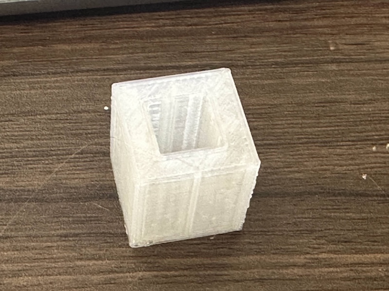Dimensions

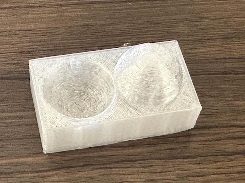surface-finish

Moreover, I added three parameters that are related to 3D printing conditions:

• filament: It represent the filament material (ex: 1=PETG, 2=PLA...)
• lastdry: It replresent how log it passed since the filament was dried (days as integer)
• model: It represent the printed object (ex: 1=Benchy, 2=dimensions, 3=surface-finish

Moreover, each printing log are filtered around actual printed time. Then, I integrated all three dataframe of printlog into one dataframe (df_integrate).

## benchy
df_temp_benchy = get_printer_temp_data('./datasets/printer_data_temperature_benchy.txt')
df_pos_benchy = get_printer_pos_data('./datasets/printer_data_position_benchy.txt')
df_benchy = pd.merge(df_pos_benchy,df_temp_benchy,on='timestamp',how="inner")
df_benchy = df_benchy.query('timestamp >= "2025/11/24 21:28:06" & timestamp <= "2025/11/24 22:14:24"')
df_benchy.loc[:,'filament'] = 1
df_benchy.loc[:,'lastdry'] = 7
df_benchy.loc[:,'model'] = 1

timestamp = df_benchy['ts_nano_x'].to_numpy()
ts_diff = np.diff(timestamp)
ts_diff = np.insert(ts_diff,0,0)
ts_sum = np.cumsum(ts_diff)
df_benchy.loc[:,'ts_sum'] = ts_sum


## dimensions
df_temp_dimensions = get_printer_temp_data('./experiments/printer_data_temp_dimensions.txt')
df_pos_dimensions = get_printer_pos_data('./experiments/printer_data_position_dimensions.txt')
df_dimensions = pd.merge(df_pos_dimensions,df_temp_dimensions,on='timestamp',how='inner')
df_dimensions = df_dimensions.query('timestamp >= "2025/12/01 10:33:50" & timestamp <= "2025/12/01 10:50:46"')
df_dimensions.loc[:,'filament'] = 1
df_dimensions.loc[:,'lastdry'] = 14
df_dimensions.loc[:,'model'] = 2

timestamp = df_dimensions['ts_nano_x'].to_numpy()
ts_diff = np.diff(timestamp)
ts_diff = np.insert(ts_diff,0,0)
ts_sum = np.cumsum(ts_diff)
df_dimensions.loc[:,'ts_sum'] = ts_sum



## finish
df_temp_finish = get_printer_temp_data('./experiments/printer_data_temp_finish.txt')
df_pos_finish = get_printer_pos_data('./experiments/printer_data_position_finish.txt')
df_finish = pd.merge(df_pos_finish,df_temp_finish,on='timestamp',how='inner')
df_finish = df_finish.query('timestamp <= "2025/12/01 11:22:50"')
df_finish.loc[:,'filament'] = 1
df_finish.loc[:,'lastdry'] = 14
df_finish.loc[:,'model'] = 3

timestamp = df_finish['ts_nano_x'].to_numpy()
ts_diff = np.diff(timestamp)
ts_diff = np.insert(ts_diff,0,0)
ts_sum = np.cumsum(ts_diff)
df_finish.loc[:,'ts_sum'] = ts_sum


df_integrate = pd.concat([df_benchy,df_dimensions,df_finish],ignore_index=True)

Visualizaiton to check

I checked whether the new added data has workd or not.... First, here is the transition of e_total($et$), represented how much extruder position totally moved through printing time.

import matplotlib.pyplot as plt

df_test_b = df_integrate.query('model == 1')
e_total_b = df_test_b['e_total'].to_numpy()

ts_sum = df_test_b['ts_sum']
plt.plot(ts_sum,e_total_b,'g-',label="3D Benchy")

df_test_dim = df_integrate.query('model == 2')
e_total_dim = df_test_dim['e_total'].to_numpy()

ts_sum_dim = df_test_dim['ts_sum']
plt.plot(ts_sum_dim,e_total_dim,'b-',label="Dimensions")

df_test_sf = df_integrate.query('model == 3')
e_total_sf = df_test_sf['e_total'].to_numpy()

ts_sum_sf = df_test_sf['ts_sum']
plt.plot(ts_sum_sf,e_total_sf,'r-',label='Surface Finish')

print(ts_sum.max(),ts_sum_dim.max(),ts_sum_sf.max())

plt.xlabel("time since print started (second)")
plt.ylabel("Total move of extruder")
plt.xlim(0.0,ts_sum.max())
plt.legend()
plt.show()

2778.0 1009.0 1292.0

I also checked the x,y positions and extruder move in time-sequence.

#--- Benchy ---#
x_pos_b = df_test_b['X_pos']
x_pos_b = x_pos_b.to_numpy()
y_pos_b = df_test_b['Y_pos']
y_pos_b = y_pos_b.to_numpy()
z_pos_b = df_test_b['Z_pos']
z_pos_b = z_pos_b.to_numpy()
e_pos_b = df_test_b['E_pos']
e_pos_b = e_pos_b.to_numpy()

#--- Dimensions ---#
x_pos_d = df_test_dim['X_pos']
x_pos_d = x_pos_d.to_numpy()

y_pos_d = df_test_dim['Y_pos']
y_pos_d = y_pos_d.to_numpy()

z_pos_d = df_test_dim['Z_pos']
z_pos_d = z_pos_d.to_numpy()

e_pos_d = df_test_dim['E_pos']
e_pos_d = e_pos_d.to_numpy()

#--- Surface Finish ---#
x_pos_f = df_test_sf['X_pos']
x_pos_f = x_pos_f.to_numpy()

y_pos_f = df_test_sf['Y_pos']
y_pos_f = y_pos_f.to_numpy()

z_pos_f = df_test_sf['Z_pos']
z_pos_f = z_pos_f.to_numpy()

e_pos_f = df_test_sf['E_pos']
e_pos_f = e_pos_f.to_numpy()

fig = plt.figure(figsize=(12,9))
fig.patch.set_facecolor('white')

fig.suptitle('x,y,z position and endeffector position')

plt.rcParams["axes.facecolor"] = 'white'
plt.rcParams["axes.edgecolor"] = 'black'
plt.subplot(3,4,1)

plt.scatter(x_pos_b,y_pos_b,c=e_pos_b,cmap="plasma",s=5)
plt.xlim(75,175)
plt.ylim(75,175)
plt.title("Benchy x_pos,y_pos")

plt.subplot(3,4,2)
plt.scatter(x_pos_b,z_pos_b,c=e_pos_b,cmap="plasma",s=5)
plt.xlim(75,180)
plt.ylim(0,75)
plt.title("Benchy x_pos,z_pos")

plt.subplot(3,4,3)
plt.scatter(y_pos_b,z_pos_b,c=e_pos_b,cmap="plasma",s=5)
plt.xlim(75,150)
plt.ylim(0,75)
plt.title("Benchy y_pos,z_pos")

plt.subplot(3,4,4)

plt.scatter(ts_sum,e_pos_b,label="e_pos",c=e_pos_b,cmap="plasma",s=10)
plt.ylim(top=120.0)
plt.ylim(bottom=-1.0)
plt.xlabel("time")
plt.ylabel("Extruder move")
plt.title("Benchy, Transition of Extruder Move")


plt.subplot(3,4,5)
plt.scatter(x_pos_d,y_pos_d,c=e_pos_d,cmap="plasma",s=5)
plt.xlim(75,175)
plt.ylim(75,175)
plt.title("Dimensions x_pos,y_pos")

plt.subplot(3,4,6)
plt.scatter(x_pos_d,z_pos_d,c=e_pos_d,cmap="plasma",s=5)
plt.xlim(75,180)
plt.ylim(0,75)
plt.title("Dimensions x_pos,z_pos")

plt.subplot(3,4,7)
plt.scatter(y_pos_d,z_pos_d,c=e_pos_d,cmap="plasma",s=5)
plt.xlim(75,150)
plt.ylim(0,75)
plt.title("Dimensions y_pos,z_pos")

plt.subplot(3,4,8)

plt.scatter(ts_sum_dim,e_pos_d,label="e_pos_d",c=e_pos_d,cmap="plasma",s=10)
plt.ylim(top=120.0)
plt.ylim(bottom=-1.0)
plt.xlabel("time")
plt.ylabel("Extruder move")
plt.title("Dimensions, Transition of Extruder Move")

plt.subplot(3,4,9)
plt.scatter(x_pos_f,y_pos_f,c=e_pos_f,cmap="plasma",s=5)
plt.xlim(75,175)
plt.ylim(75,175)
plt.title("Surface-Finish x_pos,y_pos")

plt.subplot(3,4,10)
plt.scatter(x_pos_f,z_pos_f,c=e_pos_f,cmap="plasma",s=5)
plt.xlim(75,180)
plt.ylim(0,75)
plt.title("Surface-Finish x_pos,z_pos")

plt.subplot(3,4,11)
plt.scatter(y_pos_f,z_pos_f,c=e_pos_f,cmap="plasma",s=5)
plt.xlim(75,150)
plt.ylim(0,75)
plt.title("Surface-Finish y_pos,z_pos")

plt.subplot(3,4,12)

plt.scatter(ts_sum_sf,e_pos_f,label="e_pos_f",c=e_pos_f,cmap="plasma",s=10)
plt.ylim(top=120.0)
plt.ylim(bottom=-1.0)
plt.xlabel("time")
plt.ylabel("Extruder move")
plt.title("Surface-Finish, Transition of Extruder Move")

plt.tight_layout()
plt.savefig('./notupload/viz_print.png')
plt.show()

Predict extruder move/sec ($\risingdotseq$ filament use/sec ?)

In this assignment, I am so struggle to apply neural network to printer logs, I couldn't image what log I can use for.... So, I asked ChatGPT:

In this episode, I'm having a hard time visualizing how the logs from my 3D printer could be used. I can somewhat picture it with survey data or real-world data (like predicting museum ticket sales), but where exactly could Deep Neural Networks be applied to a machine like a 3D printer?

Then, ChatGPT suggested something.... summrized as following

• Optimization of Extrusion
• Anomaly Detection
• Print Quality Prediction
• Learn the optimal settings for each material
• ... and more

... So, in this time, I decide to try prediction of extruder move (maybe it would equal with filament use) as a first test of Extrusion Optimization.

1st Machine Learning

First, I created the model that simply predict the "e_total" (total position of extruder movement) by using MLPRegressor in scikit-learn.

I choosed input variables from the position log data (X_pos, Y_pos, Z_pos, E_pos, travel_distance, e_move, ts_nano_x and set "e_total"(how mach does the extruder moved) as output variable. Then, write this code:

from sklearn.neural_network import MLPRegressor
from sklearn.preprocessing import StandardScaler
from sklearn import model_selection
import numpy as np
from datetime import datetime as dt

X = df_integrate.loc[:,['X_pos','Y_pos','travel_distance','Z_pos','E_pos','e_move','ts_nano_x']]
columns = X.columns
X = X.to_numpy()
print(X.shape)
Y = df_integrate.loc[:,['e_total']].to_numpy()
Y = np.ravel(Y)
print(Y.shape)

scaler = StandardScaler()
X = scaler.fit_transform(X)
#Y = scaler.fit_transform(Y)

X_train,X_test,y_train,y_test = model_selection.train_test_split(X,Y,test_size=0.2)

print(X_train.shape, X_test.shape,y_train.shape,y_test.shape)

model = MLPRegressor(max_iter=10000)

starttime = dt.now()
model.fit(X_train,y_train)
endtime = dt.now()
print("Predict:",model.score(X_test,y_test)," time:", (endtime.timestamp() - starttime.timestamp()))

fig,ax=plt.subplots()
fig.figsize=(10,7)
fig.patch.set_facecolor('white')

#plt.rcParams["axes.facecolor"] = 'black'
#plt.rcParams["axes.edgecolor"] = 'white'
#plt.title("Loss Curve")
ax.set_title("Loss Curve")
#plt.plot(model.loss_curve_,s=10)
ax.plot(model.loss_curve_)
#plt.xlabel("Iteration",color="white")
ax.set_xlabel("Iteration")
#plt.ylabel("Loss",color="white")
ax.set_ylabel("Loss")
ax.tick_params(axis="both")
plt.grid()
plt.savefig("./notupload/ml-1st.png")
plt.show()

(5414, 7)
(5414,)
(4331, 7) (1083, 7) (4331,) (1083,)
Predict: 0.9772217125660619  time: 11.494770050048828

the model accuracy was about 97% in 10000 iteration. It tooks 26 seconds to complete.

I created the scatter plot of predict data and real data as follow.

y_predict = model.predict(X_test)
y_real = y_test

plt.plot(y_predict,y_real,'o')
plt.xlabel("E Total Predict")
plt.ylabel("E Total Real")
plt.show()

We can use some module of scikit learn to find out which variable are important for model creation. In case of MLPRegression, we can use "permutation importance" to find it out. As following result, the most important feature for "e_total" could be "Z_position"..... It seems obvious...

from sklearn.inspection import permutation_importance

result = permutation_importance(model,X_test,y_test,n_repeats=15)
print(X_test.shape,y_test.shape)

importances = result.importances_mean
imp = pd.DataFrame()
imp['feature_name'] = columns
imp.set_index('feature_name')
imp['feature_value'] = importances
imp

(1083, 7) (1083,)

	feature_name	feature_value
0	X_pos	0.053249
1	Y_pos	0.019541
2	travel_distance	0.001945
3	Z_pos	1.503580
4	E_pos	0.028698
5	e_move	0.004863
6	ts_nano_x	0.215202

I added more fetures for learning... totally, number of feature could be 15.

from sklearn.neural_network import MLPRegressor
from sklearn.preprocessing import StandardScaler
from sklearn import model_selection
import numpy as np
from datetime import datetime as dt

X2 = df_integrate.loc[:,['X_pos','Y_pos','Z_pos','E_pos','travel_distance','e_move','hotend_temp_current','bed_temp_current','heatbreak_temp_current','hotend_power','bed_heater_power','filament','lastdry','model']]
columns2 = X2.columns

X2 = X2.to_numpy()
Y2 = df_integrate.loc[:,['e_total']].to_numpy()
Y2 = np.ravel(Y2)
scaler = StandardScaler()
X2 = scaler.fit_transform(X2)
#Y = scaler.fit_transform(Y)

X_train2,X_test2,y_train2,y_test2 = model_selection.train_test_split(X2,Y2,test_size=0.2)

model2 = MLPRegressor(max_iter=10000)

print(X_train2.shape,X_test2.shape,y_train2.shape,y_test2.shape)

starttime = dt.now()
model2.fit(X_train2,y_train2)
endtime = dt.now()
print("Predict:",model2.score(X_test2,y_test2)," Time:", (endtime.timestamp() - starttime.timestamp()))

plt.title("Loss Curve")
plt.plot(model2.loss_curve_)
plt.xlabel("Iteration")
plt.ylabel("Loss")
plt.grid()
plt.savefig('./images/ml-1st-loss-curve.png')
plt.show()

(4331, 14) (1083, 14) (4331,) (1083,)
Predict: 0.9997841842895722  Time: 10.768594026565552

Accuracy were up to 99.0%. Higher than the last model.

y_predict2 = model2.predict(X_test2)
y_real2 = y_test2

plt.scatter(y_predict2,y_real2)
plt.xlabel("E Total Predict")
plt.ylabel("E Total Real")
plt.show()

Also, checked the feature importances.

from sklearn.inspection import permutation_importance

result2 = permutation_importance(model2,X_test2,y_test2,n_repeats=15)
print(X_test2.shape,y_test2.shape)

importances2 = result2.importances_mean
imp2 = pd.DataFrame()
imp2['feature_name'] = columns2
imp2.set_index('feature_name')
imp2['feature_value'] = importances2
imp2 = imp2.sort_values('feature_value',ascending=False)
imp2 = imp2.round(4)
imp2.to_csv('./notupload/permutation-importance-1st.csv')
imp2

(1083, 14) (1083,)

	feature_name	feature_value
2	Z_pos	1.0561
12	lastdry	0.6361
13	model	0.2823
8	heatbreak_temp_current	0.0819
10	bed_heater_power	0.0161
7	bed_temp_current	0.0057
6	hotend_temp_current	0.0020
9	hotend_power	0.0018
3	E_pos	0.0002
1	Y_pos	0.0000
5	e_move	0.0000
0	X_pos	0.0000
4	travel_distance	0.0000
11	filament	0.0000

I checked the model performance with some metrics as follow:

• MAE(Mean Absolute Error)
• RMSE
• R-squared

from sklearn.metrics import mean_absolute_error,r2_score,mean_squared_error

mse = mean_absolute_error(y_real2,y_predict2)
rmse = np.sqrt(mean_squared_error(y_real2,y_predict2))

r2 = r2_score(y_real2,y_predict2)
print(f"MAE: {mse},RMSE:{rmse}, R^2:{r2}")

MAE: 12.315220619577785,RMSE:16.7304748646534, R^2:0.9997841842895722

2nd Machine Learning

I want to predict how extruder will move per second (mean how filament would be used in one second). Also, I want to expand more features with calculation.

First, I add the following variables with calculation

• difference of each x,y,z position with using numpy.diff() -> to calculate distance and speed that the position moves.
• defference of each e_total,e_move values (also using numpy.diff()

Also, Standarization and Normalization of the data is important. Beacause, for example, raw values of "e_total" (total amount of extruder movement) are too bigger than other variables, it should be normalized(should be mapped between 0 ~ 1) or standalized (should be mapped mean = 0 and std = 1).

Then, I asked ChatGPT as follow:

Write a code to create neural network model for predict extruder move in printing log. Use only jax and numpy to create the model. Input size is 15 and output size is 1.

I added the variables section, graph plot and time counter to the presented code from Chat GPT:

import numpy as np
import pandas as pd

df = df_integrate.copy()
df = df.sort_values("ts_nano_x").reset_index(drop=True)

# numpy配列に
x = df["X_pos"].to_numpy().astype(np.float32)
y = df["Y_pos"].to_numpy().astype(np.float32)
z = df["Z_pos"].to_numpy().astype(np.float32)
e = df["E_pos"].to_numpy().astype(np.float32)
t = df["ts_nano_x"].to_numpy().astype(np.float32)
f = df["filament"].to_numpy()
em = df["e_move"].to_numpy().astype(np.float32)
em = np.delete(em,0)
et = df["e_total"].to_numpy().astype(np.float32)
f = np.delete(f,0)
d = df["lastdry"].to_numpy()
d = np.delete(d,0)
m = df["model"].to_numpy()
m = np.delete(m,0)
tt = df["ts_sum"].to_numpy().astype(np.float32)
tt = np.delete(tt,0)

hotend_temp     = df["hotend_temp_current"].to_numpy().astype(np.float32)
hotend_temp     = np.delete(hotend_temp,0)

bed_temp        = df["bed_temp_current"].to_numpy().astype(np.float32)
bed_temp        = np.delete(bed_temp,0)

hotend_power    = df["hotend_power"].to_numpy().astype(np.float32)
hotend_power    = np.delete(hotend_power,0)

bed_power       = df["bed_heater_power"].to_numpy().astype(np.float32)
bed_power       = np.delete(bed_power,0)

heatbreak_temp  = df["heatbreak_temp_current"].to_numpy().astype(np.float32)
heatbreak_temp  = np.delete(heatbreak_temp,0)

dx = np.diff(x)
dy = np.diff(y)
dt = np.diff(t)
de = np.diff(e)
det_raw = np.diff(et)

dist  = np.sqrt(dx*dx + dy*dy)
eps = 1e-9

dt = np.where(dt < eps, eps ,dt)
speed = dist / dt

#ets = et / et.max()

#det_raw = np.insert(det_raw,0,0)
print(det_raw.shape)


mask = (det_raw > 0.05)
det_filt = det_raw[mask]

y_max = np.max(np.abs(det_filt))
print("det_raw min/max:", det_filt.min(), det_filt.max())
print("y_max:", y_max)


y = (det_filt / y_max).reshape(-1,1)

e_total_trim = et
e_total_norm = e_total_trim / e_total_trim.max()
e_total_norm = np.delete(e_total_norm,0)

X = np.stack([
    dist[mask],
    speed[mask],
    dx[mask],
    dy[mask],
    dt[mask],
    em[mask],
    e_total_norm[mask],
    hotend_temp[mask],
    bed_temp[mask],
    hotend_power[mask],
    bed_power[mask],
    f[mask],
    d[mask],
    m[mask],
    tt[mask]
], axis=1).astype(np.float32)

N = len(det_filt)
print("N:", N)
print("X shape:", X.shape)  # (N, 7)
print("y shape:", y.shape)  # (N, 1)

(5413,)
det_raw min/max: 0.050048828 14.420044
y_max: 14.420044
N: 3804
X shape: (3804, 15)
y shape: (3804, 1)

N = X.shape[0]
idx = np.arange(N)
np.random.seed(0)
np.random.shuffle(idx)

n_train = int(0.7 * N)
n_val   = int(0.15 * N)

idx_train = idx[:n_train]
idx_val   = idx[n_train:n_train+n_val]
idx_test  = idx[n_train+n_val:]

X_train = X[idx_train]
y_train = y[idx_train]

X_val   = X[idx_val]
y_val   = y[idx_val]

X_test  = X[idx_test]
y_test  = y[idx_test]

mean = X_train.mean(axis=0, keepdims=True)
std  = X_train.std(axis=0, keepdims=True) + 1e-6

X_train_s = (X_train - mean) / std
X_val_s   = (X_val   - mean) / std
X_test_s  = (X_test  - mean) / std

print("train:", X_train_s.shape, "val:", X_val_s.shape, "test:", X_test_s.shape)

train: (2662, 15) val: (570, 15) test: (572, 15)

import jax
import jax.numpy as jnp
from jax import random, grad, jit
from datetime import datetime as dt

input_size  = X_train_s.shape[1]   # 7
hidden1     = 32
hidden2     = 16
output_size = 1

print(input_size,hidden1,hidden2,output_size)

key = random.PRNGKey(0)

def init_params(key):
    k1, k2, k3 = random.split(key, 3)
    W1 = random.normal(k1, (input_size, hidden1)) * jnp.sqrt(2.0/input_size)
    b1 = jnp.zeros((hidden1,))
    W2 = random.normal(k2, (hidden1, hidden2)) * jnp.sqrt(2.0/hidden1)
    b2 = jnp.zeros((hidden2,))
    W3 = random.normal(k3, (hidden2, output_size)) * jnp.sqrt(2.0/hidden2)
    b3 = jnp.zeros((output_size,))
    return (W1, b1, W2, b2, W3, b3)

@jit
def forward(params, x):
    W1, b1, W2, b2, W3, b3 = params
    h1 = jnp.tanh(x @ W1 + b1)
    h2 = jnp.tanh(h1 @ W2 + b2)
    yhat = h2 @ W3 + b3
    return yhat

@jit
def loss(params, x, y):
    pred = forward(params, x)
    return jnp.mean((pred - y)**2)

@jit
def update(params, x, y, lr):
    grads = grad(loss)(params, x, y)
    return jax.tree.map(lambda p, g: p - lr * g, params, grads)

params = init_params(key)


learning_rate = 1e-3
n_steps = 30000

Xtr = jnp.array(X_train_s)
ytr = jnp.array(y_train)
Xv  = jnp.array(X_val_s)
yv  = jnp.array(y_val)

train_losses = []
val_losses = []

starttime = dt.now()
for step in range(n_steps+1):
    params = update(params, Xtr, ytr, learning_rate)
    if step % 1000 == 0:
        train_loss = loss(params, Xtr, ytr)
        val_loss   = loss(params, Xv, yv)
        print(f"step {step}  train_loss={float(train_loss)}  val_loss={float(val_loss):.4f}")
        train_losses.append(float(train_loss))
        val_losses.append(float(val_loss))
endtime = dt.now()

print(f"Finished with: {endtime.timestamp() - starttime.timestamp()} second.")

steps = np.arange(0,n_steps+1,1000)
plt.figure(figsize=(8,5))
plt.plot(steps,train_losses,label="train loss")
plt.plot(steps,val_losses,label="val loss")
plt.xlabel("step")
plt.ylabel("loss")
plt.title("Training / validation Loss")
plt.ylim(0.0,0.1)
plt.grid(True)
plt.legend()
plt.show()

15 32 16 1
step 0  train_loss=0.6885389089584351  val_loss=0.6115
step 1000  train_loss=0.07052993029356003  val_loss=0.0708
step 2000  train_loss=0.041174862533807755  val_loss=0.0437
step 3000  train_loss=0.031360819935798645  val_loss=0.0342
step 4000  train_loss=0.02620084211230278  val_loss=0.0289
step 5000  train_loss=0.022940268740057945  val_loss=0.0255
step 6000  train_loss=0.020658565685153008  val_loss=0.0230
step 7000  train_loss=0.01895139552652836  val_loss=0.0212
step 8000  train_loss=0.01761256530880928  val_loss=0.0197
step 9000  train_loss=0.01652616634964943  val_loss=0.0186
step 10000  train_loss=0.01562174130231142  val_loss=0.0176
step 11000  train_loss=0.01485376339405775  val_loss=0.0168
step 12000  train_loss=0.014191576279699802  val_loss=0.0160
step 13000  train_loss=0.013613236136734486  val_loss=0.0154
step 14000  train_loss=0.013102886267006397  val_loss=0.0149
step 15000  train_loss=0.012648503296077251  val_loss=0.0144
step 16000  train_loss=0.012240895070135593  val_loss=0.0139
step 17000  train_loss=0.011872739531099796  val_loss=0.0135
step 18000  train_loss=0.011538325808942318  val_loss=0.0132
step 19000  train_loss=0.01123297680169344  val_loss=0.0129
step 20000  train_loss=0.010952918790280819  val_loss=0.0126
step 21000  train_loss=0.010694766417145729  val_loss=0.0123
step 22000  train_loss=0.010456003248691559  val_loss=0.0121
step 23000  train_loss=0.01023426465690136  val_loss=0.0118
step 24000  train_loss=0.010027710348367691  val_loss=0.0116
step 25000  train_loss=0.00983464252203703  val_loss=0.0114
step 26000  train_loss=0.009653686545789242  val_loss=0.0112
step 27000  train_loss=0.009483621455729008  val_loss=0.0111
step 28000  train_loss=0.009323401376605034  val_loss=0.0109
step 29000  train_loss=0.009172014892101288  val_loss=0.0107
step 30000  train_loss=0.009028837084770203  val_loss=0.0106
Finished with: 12.652096033096313 second.

Then, I also asked ChatGPT:

Write a code to evaluate the performance of the model. Use metrics MAE, RMSE, R-square for evaluation. Also please make a graphs plotting prediction and true data. The graph should be created both scealed and real data.

from sklearn.metrics import mean_absolute_error, r2_score
from math import sqrt

Xt_s = jnp.array(X_test_s) 
yt_s = jnp.array(y_test)   

y_pred_s = forward(params, Xt_s) 

y_true_s = np.array(yt_s).reshape(-1)     
y_pred_s = np.array(y_pred_s).reshape(-1)

MAE  = mean_absolute_error(y_true_s, y_pred_s)
RMSE = np.sqrt(((y_true_s - y_pred_s)**2).mean())
R2   = r2_score(y_true_s, y_pred_s)

print("MAE (scaled) :", MAE)
print("RMSE (scaled):", RMSE)
print("R^2 (scaled) :", R2)

plt.figure(figsize=(6,6))
plt.scatter(y_true_s, y_pred_s, s=5, alpha=0.3)
plt.xlabel("true ΔEtotal (scaled)")
plt.ylabel("predicted ΔEtotal (scaled)")
plt.axis("equal")
plt.grid(True)
plt.show()

y_true = y_true_s * float(y_max) 
y_pred = y_pred_s * float(y_max)

MAE_real  = mean_absolute_error(y_true, y_pred)
RMSE_real = np.sqrt(((y_true - y_pred)**2).mean())
R2_real   = r2_score(y_true, y_pred)

print("MAE (real) :", MAE_real)
print("RMSE(real):", RMSE_real)
print("R^2 (real):", R2_real)

print("y_true_s:", y_true_s.min(), y_true_s.max(), y_true_s.shape)
print("y_pred_s:", y_pred_s.min(), y_pred_s.max(), y_pred_s.shape)
print("y_max:", y_max)


plt.figure(figsize=(6,6))
plt.scatter(y_true, y_pred, s=5, alpha=0.3)
plt.xlabel("true ΔEtotal")
plt.ylabel("predicted ΔEtotal")
plt.axis("equal")
plt.grid(True)
plt.show()

MAE (scaled) : 0.06407865881919861
RMSE (scaled): 0.09894792
R^2 (scaled) : 0.5007976293563843

MAE (real) : 0.9240170121192932
RMSE(real): 1.4268333
R^2 (real): 0.5007977485656738
y_true_s: 0.003470782 1.0 (572,)
y_pred_s: -0.4250085 0.6636933 (572,)
y_max: 14.420044

Outcome

In this assignment, I tried to make an machine learning model from my Prusa Core One Printer Log. I have ever created the Convolutional Neural Network models for image classification by PyTorch, but I have not so much tried to make a neural network for regression. Moreover, I am really struggled to apply neural network to my Core One 3D Printer log.... It would be very exciting time.

After finished this assignment, I wanted to add more data and integrate with the printer log. One possible final project is to make something like an emulator of my Prusa Core one based on the print log. The input would be G-Code data for print, and output data is the prediction of the printer works that represented as the format of printer log....