Naldi Carrion - Fab Lab ESAN - Fab Futures - Data Science

Home About

< Home

Week 2 - 2nd Class: Machine Learning

This class aim was to learn about neural networks, a Machine Learning model, inspire in how human brain functions or operate. Thus, it requieres a complex math model that learn patterns to:

• Recognise images
• Forecasting
• Classify text, images, behaviors
• To take decisions base on data Hence, it could be a simple math model base on a simple algortihm or a complex model with several different algorithms, which receive data and process them to generate an output.

Neural networks components

• Imput Layer (Capa de entrada): Receive data as imput
• Hidden Layers (Capas ocultas): Layers where different models run and patterns are learned, more complex the model more hidden layers we will have
• Output Layer (Capa de salida): Final output (a number, regresion, binary classification, or several categories)

Activation functions

Once the neural network receive data, it will process diferent functions, algorithms or models and it will need to apply a special function to learn patterns, this function is called "activation funtion". This function act as a filter, transforming data, allowing the neural network to learn. During the class the professor mention the following:

• Sigmoid: Tranform any number in a value between 0 and 1, use in probability
• Tanh: Tranform any number in a value between -1 and 1
• ReLU (Rectified Linear Unit - Unidad Lineal Rectificada): Nowdays highly use, transfor every negative valu to 0; kepping the positive ones, the problem is that vanishing gradients could occur.
• Leaky ReLU: Similar to ReLU, however allows to get some negative imputs assigning a small positive gradient to avoid vanishing gradients.

How a neural network learn?

Through backpropagation, the training process is a cycle (loop): imput → prediction → compare prediction with real value → error calculation → internal parameters adjustment → feedback loop. It is like learning something and try out, if we fail, we will try again, that is backpropagation (correcting error). This algorithm propagates errors back through the network to generate weight updates. Concepts that we need to understand:

• Gradient descent: The way weights are adjusted to reduce loss function
• Learning rate: Proportion (ratio) at which gradients are applied to update weights

Optimization Algorithm

Method use to decide how the network could be adjust when an error is detected. During the class professor highlithed:

• Stochastic gradient descent (SGD): Classic method, adjust step by step the weights on random subsets.
• Adam (Adaptive Moment Estimation): Adjust learning rate correcting error anticipating how error curve is "moving"

Overfitting

This occurs when the model learns the dataset so perfectly that it no longer generalizes (like memorizing an exam instead of learning the material). Techniques to prevent this:

• Dropout: randomly shuts down neurons while training
• Early stopping: halts training when it no longer improves
• Regularization: adds penalties to prevent the model from becoming overly complex

Type of networks

• MLP / DNN (Multi-Layer Perceptron / Deep Neural Network) = “Common” interconnected layered networks, use them for:
  • Basic classification
  • Regression
  • Training with tabular data
  • Simple pattern recognition
• CNN (Convolutional Neural Network) = Detect visual patterns such as edges, curves, shapes and others forms. They mimic how the human eye works, we can use it for:
  • Images
  • Computer vision
  • Object detection
  • Facial recognition
  • Meter reading
• RNN / LSTM (Recurrent Neural Network / Long Short-Term Memory) = Use to read and analyse data such as:
  • Text
  • Sentences
  • Time series
  • Sequential data
  • Predicting future values
• GAN (Generative Adversarial Network) = Generate images or videos, the model is composed of two competing networks:
  • Generator: creates fake images
  • Discriminator: attempts to detect them Purposes:
  • Generate realistic images
  • Create synthetic videos
  • Deepfakes
  • Improve resolution
  • Create art
  • Fill in missing images
• Transformers / LLMs (Large Language Models) = like Chat GPT, Gemini and other, use to:
  • Understand and generate text
  • Translating
  • Reasoning
  • Summarizing
  • Performing complex language-based tasks
  • And today also images, audio, etc.
• VAE (Variational Autoencoder) = Data generation and compression, an autoencoder is like shrinking the image to a very small representation (encoding) and expanding it back to its original form (decoding), if done correctly, it can create new images similar to the originals. USe it to:
  • Generate new images
  • Reduce dimensionality
  • Reconstruct data
  • Detect anomalies

Assignment

Water Meter Image Project – Machine Learning Notebook

This notebook summarizes the work project where I trained a Machine Learning model to read the red decimal digits of a water meter from images.

The goal is to build a clear, reproducible pipeline that I can use in my final presentation:

• Load and clean the labels from a CSV file
• Verify consistency between CSV labels and image files
• Preprocess images (grayscale, resize, normalize)
• Train a Random Forest regression model using flattened images
• Evaluate performance with Mean Absolute Error (MAE)
• Visualize sample predictions and images for interpretation

I want to train a Machine Learning model to automatically recognize the decimal digits (the red ones) of a water meter from images that we have for a project. This perfectly fulfills the requirement of "fitting a machine learning model to your data" because:

• I have real data (400 images)
• They are partially labeled (correct digit in an Excel file), only number in red (last numbers of a the water meter)
• The problem is clear: predicting a numeric value between 0 and 999 from each image (a regression problem), where the label corresponds to the last three red digits of the water meter

• Step 0. Problem Description I have photos of the red digits on a water meter, each image contains a group of digits that runs from 0 to 9. The goal is to train a model that, given a photo, predicts the correct digit. This will serve as part of a system to automatically monitor water consumption.

  

1. Setup and libraries

import os

import numpy as np
import pandas as pd

from PIL import Image
import matplotlib.pyplot as plt

from sklearn.model_selection import train_test_split
from sklearn.ensemble import RandomForestRegressor
from sklearn.metrics import mean_absolute_error

# Show plots inside Jupyter
%matplotlib inline

plt.rcParams['figure.figsize'] = (6, 4)

2. Problem description

I work with 400+ images from a real water-meter monitoring project.

• Each image shows the red decimal digits of the meter (from 000 to 999).
• A CSV file contains the correct 3-digit reading for each image.
• The task is to predict the numeric value (between 0 and 999) from each image.
• This is treated as a regression problem (predicting a number, not a class).

If the model performs well, it can be integrated in a real system to automatically read water meters from photos.

3. Loading and cleaning labels

The labels are stored in:

• File: datasets/3rd_Class_Assignment/Etiqueta_Rojo_V2.csv
• Columns of interest:
  • Image: image file name (without extension at the beginning)
  • label: correct reading of the red digits

Steps:

1. Read the CSV, keeping only Image and label.
2. Drop rows with missing values.
3. Clean and convert label to integer.
4. Standardize image names (lowercase + .jpeg).

• Step 1. Read the labels from CSV I will use only the "Reds" sheet from the Label_V2.csv file.

import pandas as pd

df = pd.read_csv("datasets/3rd_Class_Assignment/Etiqueta_Rojo_V2.csv", sep=";")
df = df.loc[:, ["Image", "label"]]
df.head()

	Image	label
0	Picture 1 (1)	863.0
1	Picture 1 (2)	863.0
2	Picture 1 (3)	863.0
3	Picture 1 (4)	863.0
4	Picture 1 (5)	863.0

• Step 2. Drop rows with missing values & Step 3. Clean and convert label to integer Including zeros at the right side

import pandas as pd

# Leer el CSV
df = pd.read_csv(
    "datasets/3rd_Class_Assignment/Etiqueta_Rojo_V2.csv",
    sep=";"
)

# Nos quedamos solo con las columnas correctas
df = df.loc[:, ["Image", "label"]]

# Limpiamos la columna 'label'
df["label"] = df["label"].astype(str)       # todo a texto
df["label"] = df["label"].str.strip()      # quitar espacios
df = df[df["label"] != ""]                 # eliminar vacíos
df["label"] = pd.to_numeric(df["label"], errors="coerce")
df = df.dropna(subset=["label"])           # eliminar errores
df["label"] = df["label"].astype(int)      # ahora sí, enteros

df.head(), df.dtypes

(           Image  label
 0  Picture 1 (1)    863
 1  Picture 1 (2)    863
 2  Picture 1 (3)    863
 3  Picture 1 (4)    863
 4  Picture 1 (5)    863,
 Image    object
 label     int64
 dtype: object)

• Step 4. Standardize image names (lowercase + .jpeg).

# Eliminar repeticiones múltiples de ".jpeg"
while df["Image"].str.contains(".jpeg.jpeg").any():
    df["Image"] = df["Image"].str.replace(".jpeg.jpeg", ".jpeg", regex=False)

df.head()

	Image	label
0	picture 1 (1).jpeg	863
1	picture 1 (2).jpeg	863
2	picture 1 (3).jpeg	863
3	picture 1 (4).jpeg	863
4	picture 1 (5).jpeg	863

# NORMALIZAR NOMBRES DE ARCHIVOS DEL CSV
# Normalizar nombres de archivo SIN agregar extensiones
df["Image"] = df["Image"].astype(str).str.strip().str.lower()

df.head()

	Image	label
0	picture 1 (1).jpeg	863
1	picture 1 (2).jpeg	863
2	picture 1 (3).jpeg	863
3	picture 1 (4).jpeg	863
4	picture 1 (5).jpeg	863

4. Consistency check between CSV and image folder

Before training any model, it is important to ensure that:

• Every image mentioned in the CSV file exists in the image folder
• There are no extra images without labels

This step avoids silent errors during training and evaluation.

import os

image_dir = "datasets/3rd_Class_Assignment/Rojo_V2"

# Listado real de archivos en la carpeta
folder_files = set(os.listdir(image_dir))

# Listado de archivos según el CSV
csv_files = set(df["Image"].tolist())

# Archivos que están en CSV pero NO en la carpeta
missing_files = csv_files - folder_files

# Archivos que están en carpeta pero NO en CSV
extra_files = folder_files - csv_files

print("Faltan estos archivos (CSV → carpeta):")
print(missing_files)

print("\nSobran estos archivos (carpeta → CSV):")
print(extra_files)

Faltan estos archivos (CSV → carpeta):
set()

Sobran estos archivos (carpeta → CSV):
set()

# Filas donde Image es NaN
empty_nan = df[df["Image"].isna()]

# Filas donde Image no es NaN pero está vacía después de limpiar
empty_blank = df[df["Image"].astype(str).str.strip() == ""]

print("Filas con NaN:")
print(empty_nan)

print("\nFilas con texto vacío:")
print(empty_blank)

Filas con NaN:
Empty DataFrame
Columns: [Image, label]
Index: []

Filas con texto vacío:
Empty DataFrame
Columns: [Image, label]
Index: []

import pandas as pd

# Leer el CSV
df = pd.read_csv("datasets/3rd_Class_Assignment/Etiqueta_Rojo_V2.csv", sep=";")

# Nos quedamos solo con las columnas correctas
df = df.loc[:, ["Image", "label"]]

# 1) Eliminar filas donde Image o label son NaN (las vacías del final)
df = df.dropna(subset=["Image", "label"])

# 2) Resetear el índice para que quede limpio
df = df.reset_index(drop=True)

df.head(), df.shape

(           Image  label
 0  Picture 1 (1)  863.0
 1  Picture 1 (2)  863.0
 2  Picture 1 (3)  863.0
 3  Picture 1 (4)  863.0
 4  Picture 1 (5)  863.0,
 (442, 2))

Clean and convert label to integer:

df["label"] = df["label"].astype(str)
df["label"] = df["label"].str.strip()
df["label"] = pd.to_numeric(df["label"], errors="coerce")
df = df.dropna(subset=["label"])
df["label"] = df["label"].astype(int)

Standardize image names:

df["Image"] = df["Image"].str.lower() + ".jpeg"

import os

image_dir = "datasets/3rd_Class_Assignment/Rojo_V2"

folder_files = set(os.listdir(image_dir))
csv_files = set(df["Image"].tolist())

missing_files = csv_files - folder_files
extra_files = folder_files - csv_files

print("Faltan estos archivos (CSV → carpeta):", missing_files)
print("Sobran estos archivos (carpeta → CSV):", extra_files)

Faltan estos archivos (CSV → carpeta): set()
Sobran estos archivos (carpeta → CSV): set()

5. Loading and preprocessing images

For each row in the cleaned DataFrame:

1. Open the corresponding image from Rojo_V2
2. Convert to grayscale
3. Resize to 64 × 64 pixels
4. Normalize pixel values to the range [0, 1]
5. Store image as a NumPy array, and store its label

Finally:

• X will contain all images
• y will contain the corresponding 3-digit labels

import numpy as np
from PIL import Image
import os

image_dir = "datasets/3rd_Class_Assignment/Rojo_V2"

X = []
y = []

for _, row in df.iterrows():
    filename = row["Image"]
    label = row["label"]

    img_path = os.path.join(image_dir, filename)

    try:
        # Cargar imagen y convertir a escala de grises
        img = Image.open(img_path).convert("L")

        # Redimensionar a 64x64
        img = img.resize((64, 64))

        # Normalizar a rango [0, 1]
        X.append(np.array(img) / 255.0)
        y.append(label)

    except Exception as e:
        print("Error al cargar:", img_path, " → ", e)

# Convertir a arrays numpy
X = np.array(X, dtype="float32")
y = np.array(y, dtype="float32")

# Añadir canal para CNN: (N, 64, 64, 1)
X = X[..., np.newaxis]

X.shape, y.shape

((442, 64, 64, 1), (442,))

6. Preparing data for a classical ML model

I use a Random Forest Regressor, which expects 2D input:

• Shape: (n_samples, n_features)

So I flatten each image from (64, 64, 1) into a single vector of length 4096.

# X tiene forma (n_imágenes, 64, 64, 1)
X_flat = X.reshape((X.shape[0], -1))
X_flat.shape

(442, 4096)

7. Train–test split

I split the dataset into:

• Training set: 80% of the images
• Test set: 20% of the images

The test set is kept separate to obtain an unbiased estimate of model performance.

from sklearn.model_selection import train_test_split

X_train, X_test, y_train, y_test = train_test_split(
    X_flat, y, test_size=0.2, random_state=42
)

X_train.shape, X_test.shape, y_train.shape, y_test.shape

((353, 4096), (89, 4096), (353,), (89,))

8. Training a Random Forest regression model

I chose a Random Forest Regressor because:

• It is robust to noise and works well with tabular data (flattened pixels)
• It can model non-linear relationships
• It requires very little hyperparameter tuning for a good baseline

Key settings:

• n_estimators = 300 trees
• random_state = 42 for reproducibility
• n_jobs = -1 to use all CPU cores available

from sklearn.ensemble import RandomForestRegressor

rf_model = RandomForestRegressor(
    n_estimators=300,
    random_state=42,
    n_jobs=-1
)

rf_model.fit(X_train, y_train)
print("Modelo entrenado.")

Modelo entrenado.

9. Model evaluation – Mean Absolute Error (MAE)

To evaluate the model, I use Mean Absolute Error (MAE):

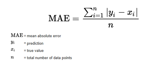
In our case:

• y_i = true meter reading
• ŷ_i = predicted reading
• N = number of samples

MAE tells us, on average, how many units the prediction is off from the true value.

from sklearn.metrics import mean_absolute_error

y_pred = rf_model.predict(X_test)
mae = mean_absolute_error(y_test, y_pred)

print("MAE =", mae)

MAE = 3.0522846441947586

Model Evaluation – Interpretation (MAE)

To evaluate the performance of the model, I used the Mean Absolute Error (MAE), which measures the average difference between the true meter reading and the predicted value. The model achieved:

MAE = 3.05

This means that, on average, the model is off by only 3 units when predicting the 3-digit value (000–999) shown in the red digits of the water meter. Considering the restricted dataset size (442 labeled images) and the classical machine learning approach (Random Forest), I think that this is an excellent result. An average error of 3 units represents less than 0.3% deviation, which is sufficiently accurate for a real-world monitoring system where readings change gradually over time.

9.1 True vs predicted readings

A simple scatter plot of true vs predicted values helps us see the global behaviour:

• Points close to the diagonal line indicate good predictions
• Systematic deviations would appear as visible patterns

'y_test' in globals(), 'y_pred' in globals()

(True, True)

plt.figure()
plt.scatter(y_test, y_pred)
plt.xlabel("True Reading")
plt.ylabel("Predicted Reading")
plt.title("True vs Predicted Water Meter Readings")
plt.show()

10. Example predictions (numeric)

To make the result more intuitive, I round the predictions to the nearest integer and compare some examples.

import numpy as np

y_pred_round = np.round(y_pred).astype(int)

for i in range(10):
    print(f"Real: {int(y_test[i])} | Predicho: {y_pred_round[i]}")

Real: 862 | Predicho: 862
Real: 861 | Predicho: 860
Real: 872 | Predicho: 871
Real: 804 | Predicho: 828
Real: 872 | Predicho: 872
Real: 760 | Predicho: 781
Real: 821 | Predicho: 822
Real: 815 | Predicho: 817
Real: 863 | Predicho: 862
Real: 880 | Predicho: 880

# Round predictions to nearest integer
y_pred_round = np.round(y_pred).astype(int)

# Show a few examples
n_examples = 10
print("Sample comparisons (true vs predicted):\n")
for i in range(n_examples):
    print(f"True: {int(y_test[i])}  |  Predicted: {y_pred_round[i]}")

Sample comparisons (true vs predicted):

True: 862  |  Predicted: 862
True: 861  |  Predicted: 860
True: 872  |  Predicted: 871
True: 804  |  Predicted: 828
True: 872  |  Predicted: 872
True: 760  |  Predicted: 781
True: 821  |  Predicted: 822
True: 815  |  Predicted: 817
True: 863  |  Predicted: 862
True: 880  |  Predicted: 880

11. Visual examples – test images with predictions

Finally, I display some test images with their true and predicted labels in the title.

This is a powerful way to show the model’s performance in the final presentation, because the audience can see the digits and the prediction at the same time.

import matplotlib.pyplot as plt

for i in range(5):
    plt.imshow(X_test[i].reshape(64,64), cmap="gray")
    plt.title(f"Real: {int(y_test[i])} | Predicted: {y_pred_round[i]}")
    plt.axis("off")
    plt.show()

# Show a few test images with their predictions
n_images_to_show = 5

for i in range(n_images_to_show):
    img = X_test[i].reshape(64, 64)
    true_val = int(y_test[i])
    pred_val = y_pred_round[i]

    plt.figure()
    plt.imshow(img, cmap="gray")
    plt.title(f"True: {true_val}  |  Predicted: {pred_val}")
    plt.axis("off")
    plt.show()

12. Interpretation notes

When I present this notebook, I can highlight:

• Real-world data: 400+ real images from a water meter monitoring project
• Clean data pipeline: label cleaning, file consistency checks, and systematic image preprocessing
• Model performance:
  • The MAE is low compared to the full 0–999 range
  • In practical terms, the model is usually off by only a few units
• Practical relevance:
  • Such a model can support automatic meter reading, reducing manual work
  • It is a solid baseline that can later be improved with Convolutional Neural Networks (CNNs)