< Home
Week 4: Machine Learning
What I learned
・These are some curve for machine learning.
import numpy as np
import matplotlib.pyplot as plt
x = np.linspace(-3,3,100)
plt.plot(x,1/(1+np.exp(-x)),label='sigmoid')
plt.plot(x,np.tanh(x),label='tanh')
plt.plot(x,np.where(x < 0,0,x),label='ReLU')
plt.plot(x,np.where(x < 0,0.1*x,x),'--',label='leaky ReLU')
plt.legend()
plt.show()

・Also Neil suggested Jax, taht is a powerfull framework.
Practrice
In this class, Neil showed us the example of MIST mashine learning. So I tried to start his example code.
from sklearn.neural_network import MLPClassifier
import numpy as np
import matplotlib.pyplot as plt
xtrain = np.load('../class/datasets/MNIST/xtrain.npy')
ytrain = np.load('../class/datasets/MNIST/ytrain.npy')
xtest = np.load('../class/datasets/MNIST/xtest.npy')
ytest = np.load('../class/datasets/MNIST/ytest.npy')
print(f"read {xtrain.shape[1]} byte data records, {xtrain.shape[0]} training examples, {xtest.shape[0]} testing examples\n")
classifier = MLPClassifier(solver='adam',hidden_layer_sizes=(100),activation='relu',random_state=1,verbose=True,tol=0.05)
classifier.fit(xtrain,ytrain)
print(f"\ntest score: {classifier.score(xtest,ytest)}\n")
predictions = classifier.predict(xtest)
fig,axs = plt.subplots(1,5)
for i in range(5):
    axs[i].imshow(np.reshape(xtest[i],(28,28)))
    axs[i].axis('off')
    axs[i].set_title(f"predict: {predictions[i]}")
plt.tight_layout()
plt.show()
read 784 byte data records, 60000 training examples, 10000 testing examples

Iteration 1, loss = 3.36992820
Iteration 2, loss = 1.13264743
Iteration 3, loss = 0.67881655
Iteration 4, loss = 0.44722907
Iteration 5, loss = 0.31658618
Iteration 6, loss = 0.23506685
Iteration 7, loss = 0.19331921
Iteration 8, loss = 0.15768276
Iteration 9, loss = 0.13673548
Iteration 10, loss = 0.12379790
Iteration 11, loss = 0.10733766
Iteration 12, loss = 0.11199584
Iteration 13, loss = 0.09769195
Iteration 14, loss = 0.09220702
Iteration 15, loss = 0.09282348
Iteration 16, loss = 0.08964422
Iteration 17, loss = 0.08613192
Training loss did not improve more than tol=0.050000 for 10 consecutive epochs. Stopping.

test score: 0.9548

from sklearn.neural_network import MLPClassifier
import numpy as np
xtrain = np.load('../class/datasets/MNIST/xtrain.npy')
ytrain = np.load('../class/datasets/MNIST/ytrain.npy')
xtest = np.load('../class/datasets/MNIST/xtest.npy')
ytest = np.load('../class/datasets/MNIST/ytest.npy')
print(f"read {xtrain.shape[1]} byte data records, {xtrain.shape[0]} training examples, {xtest.shape[0]} testing examples\n")
classifier = MLPClassifier(solver='adam',hidden_layer_sizes=(100),activation='relu',random_state=1,verbose=True,tol=0.05)
classifier.fit(xtrain,ytrain)
print(f"\ntest score: {classifier.score(xtest,ytest)}\n")
predictions = classifier.predict(xtest)
fig,axs = plt.subplots(1,5)
for i in range(5):
    axs[i].imshow(np.reshape(xtest[i],(28,28)))
    axs[i].axis('off')
    axs[i].set_title(f"predict: {predictions[i]}")
plt.tight_layout()
plt.show()
read 784 byte data records, 60000 training examples, 10000 testing examples

Iteration 1, loss = 3.36992820
Iteration 2, loss = 1.13264743
Iteration 3, loss = 0.67881655
Iteration 4, loss = 0.44722907
Iteration 5, loss = 0.31658618
Iteration 6, loss = 0.23506685
Iteration 7, loss = 0.19331921
Iteration 8, loss = 0.15768276
Iteration 9, loss = 0.13673548
Iteration 10, loss = 0.12379790
Iteration 11, loss = 0.10733766
Iteration 12, loss = 0.11199584
Iteration 13, loss = 0.09769195
Iteration 14, loss = 0.09220702
Iteration 15, loss = 0.09282348
Iteration 16, loss = 0.08964422
Iteration 17, loss = 0.08613192
Training loss did not improve more than tol=0.050000 for 10 consecutive epochs. Stopping.

test score: 0.9548
Assignment
Fit a machine learning model to your data
At first I don't know where should I start to ask to LLM, Gemini
I want to practice deep learning using this data.
Can you think of anything interesting we could do with this data?

ID - Unique number for each athlete;
Name - Athlete's name;
Sex - M or F;
Age - Integer;
Height - In centimeters;
Weight - In kilograms;
Team - Team name;
NOC - National Olympic Committee 3-letter code;
Games - Year and season;
Year - Integer;
Season - Summer or Winter;
City - Host city;
Sport - Sport;
Event - Event;
Medal - Gold, Silver, Bronze, or NA.
import numpy as np
import matplotlib.pyplot as plt
import pandas as pd
import seaborn as sns

import os
print(os.listdir("datasets"))

#import datasets
data = pd.read_csv('datasets/olympic_athlete_events.csv')
regions = pd.read_csv('datasets/olympic_noc_regions.csv')

merged = pd.merge(data, regions, on='NOC', how='left')
['olympic_athlete_events.csv', 'factory_sensor_simulator_2040.csv', 'olympic_noc_regions.csv', '.gitignore']
goldMedals = merged[(merged.Medal == 'Gold')]
goldMedals = goldMedals.sort_values(by="Age", ascending=False)
goldMedals.head()

goldMedals.isnull().any()

#plt.figure(figsize=(50, 10))
clean_age = goldMedals['Age'].dropna().astype(int)
age_counts = clean_age.value_counts().sort_index()
x = age_counts.index
y = age_counts.values

plt.plot(x,y,'o')
#plt.figure(figsize=(8, 5))
plt.title("Olympic gold medalist vs age")
plt.xlabel("Age")
plt.ylabel("Gold medalist Count")
plt.grid(True)
plt.tight_layout()
plt.show()

1. Data Preprocessing
First, I converted the data into numerical format (NumPy arrays) compatible with JAX using Pandas and Scikit-Learn.
import pandas as pd
import numpy as np
from sklearn.preprocessing import LabelEncoder, StandardScaler
from sklearn.model_selection import train_test_split

df = pd.read_csv('datasets/olympic_athlete_events.csv')

# --- pre processing ---

# 1. dependant variable: having medal 1, NA 0
df['Target'] = df['Medal'].apply(lambda x: 0 if pd.isna(x) else 1)

# 2. convert Categorical variable into numerical variable
# Sex, NOC, Sport will be 0, 1, 2...(should be integer)
cat_cols = ['Sex', 'NOC', 'Sport', 'Season']
for col in cat_cols:
    le = LabelEncoder()
    df[col] = le.fit_transform(df[col].astype(str))

# 3. Imputation and Normalization of Missing Values in Numeric Variables
num_cols = ['Age', 'Height', 'Weight']
df[num_cols] = df[num_cols].fillna(df[num_cols].mean())
scaler = StandardScaler()
df[num_cols] = scaler.fit_transform(df[num_cols])

# 4. Split data for JAX/Flax
# Separate category input (x_cat) and numeric input (x_num).
X_cat = df[cat_cols].values  #  (int32)
X_num = df[num_cols].values  #  (float32)
y = df['Target'].values      #

# Split into training and testing sets
X_cat_train, X_cat_test, X_num_train, X_num_test, y_train, y_test = train_test_split(
    X_cat, X_num, y, test_size=0.2, random_state=42
)

# Number of unique items per category (required to determine the input size of the Embedding layer)
vocab_sizes = [df[c].max() + 1 for c in cat_cols]
df.head()
| ID | Name | Sex | Age | Height | Weight | Team | NOC | Games | Year | Season | City | Sport | Event | Medal | Target | |
|---|---|---|---|---|---|---|---|---|---|---|---|---|---|---|---|---|
| 0 | 1 | A Dijiang | 1 | -0.247880 | 5.023699e-01 | 0.739392 | China | 41 | 1992 Summer | 1992 | 0 | Barcelona | 8 | Basketball Men's Basketball | NaN | 0 |
| 1 | 2 | A Lamusi | 1 | -0.407095 | -5.754389e-01 | -0.851107 | China | 41 | 2012 Summer | 2012 | 0 | London | 32 | Judo Men's Extra-Lightweight | NaN | 0 |
| 2 | 3 | Gunnar Nielsen Aaby | 1 | -0.247880 | 3.063317e-15 | 0.000000 | Denmark | 55 | 1920 Summer | 1920 | 0 | Antwerpen | 24 | Football Men's Football | NaN | 0 |
| 3 | 4 | Edgar Lindenau Aabye | 1 | 1.344262 | 3.063317e-15 | 0.000000 | Denmark/Sweden | 55 | 1900 Summer | 1900 | 0 | Paris | 61 | Tug-Of-War Men's Tug-Of-War | Gold | 1 |
| 4 | 5 | Christine Jacoba Aaftink | 0 | -0.725523 | 1.041274e+00 | 0.898442 | Netherlands | 145 | 1988 Winter | 1988 | 1 | Calgary | 53 | Speed Skating Women's 500 metres | NaN | 0 |
Before I define the model, I installed "flax" from terminal.

Then, I tried to define the model.
2. Model Definition (Flax)
This is the core component of JAX/Flax. Using nn.Module, we create an architecture that passes categorical variables through an embedding layer and concatenates them with numerical variables.
import jax
import jax.numpy as jnp
from flax import linen as nn
import optax

class OlympicModel(nn.Module):
    vocab_sizes: list  # Number of words per category (e.g., 200 for 200 countries)
    emb_dim: int = 10  # Embedded vector dimension

    @nn.compact
    def __call__(self, x_cat, x_num):
        # 1. Handling Categorical Variables (Embedding)
        # x_cat is of shape [batch_size, 4] (Sex, NOC, Sport, Season)
        embs = []
        for i, vocab_size in enumerate(self.vocab_sizes):
            # Create an embedding layer for each category
            # Input: Integer index -> Output: 10-dimensional vector
            emb = nn.Embed(num_embeddings=vocab_size, features=self.emb_dim, name=f'emb_{i}')(x_cat[:, i])
            embs.append(emb)

        # Concatenate Embedded Vectors [batch_size, 4 * 10]
        x_emb = jnp.concatenate(embs, axis=1)

        # 2. Numeric Variables and Concatenation
        # [batch_size, 40] + [batch_size, 3] -> [batch_size, 43]
        x = jnp.concatenate([x_emb, x_num], axis=1)

        # --- 3. Fully connected layer (MLP) ---
        x = nn.Dense(features=64)(x)
        x = nn.relu(x)
        x = nn.Dense(features=32)(x)
        x = nn.relu(x)
        x = nn.Dense(features=1)(x) # 出力は1つ (Logits)

        return x
3. Defining Learning Steps (JAX Transformation)
We utilize JAX's distinctive features: jax.jit (Just-In-Time compilation) and jax.value_and_grad (automatic differentiation).
# TrainState: A class that holds the model parameters and optimizer state
from flax.training import train_state

def create_train_state(rng, learning_rate, vocab_sizes, sample_cat, sample_num):
    model = OlympicModel(vocab_sizes=vocab_sizes)
    # tx = optax.adam(learning_rate) (init)
    params = model.init(rng, sample_cat, sample_num)['params']
    tx = optax.adam(learning_rate)
    return train_state.TrainState.create(apply_fn=model.apply, params=params, tx=tx)

@jax.jit
def train_step(state, x_cat, x_num, y):
    def loss_fn(params):
        logits = state.apply_fn({'params': params}, x_cat, x_num)
        # Binary cross-entropy error (including sigmoid)
        loss = optax.sigmoid_binary_cross_entropy(logits, y.reshape(-1, 1)).mean()
        return loss

    # Simultaneously calculate loss and gradient
    loss, grads = jax.value_and_grad(loss_fn)(state.params)
    # Parameter update with the optimizer
    state = state.apply_gradients(grads=grads)
    return state, loss
4. Execution Loop
This is where the actual learning process runs.
# Initialize
rng = jax.random.PRNGKey(0)
learning_rate = 0.001
state = create_train_state(rng, learning_rate, vocab_sizes, X_cat_train[:1], X_num_train[:1])

# Simplified Learning Loop (Batch processing omitted; demo uses entire dataset)
# Mini-batch learning should be used in practice
epochs = 100

print("Training Start...")
for epoch in range(epochs):
    # Large batch sizes may cause an OutOfMemoryError, so please use DataLoader in actual production
    # This is simplified for testing purposes only
    state, loss = train_step(state, X_cat_train, X_num_train, y_train)

    if epoch % 10 == 0:
        print(f"Epoch: {epoch}, Loss: {loss:.4f}")

print("Training Finished!")
Training Start...
Epoch: 0, Loss: 0.7669
Epoch: 10, Loss: 0.6165
Epoch: 20, Loss: 0.5129
Epoch: 30, Loss: 0.4443
Epoch: 40, Loss: 0.4186
Epoch: 50, Loss: 0.4133
Epoch: 60, Loss: 0.4068
Epoch: 70, Loss: 0.4023
Epoch: 80, Loss: 0.3989
Epoch: 90, Loss: 0.3956
Training Finished!
I could see the process that decreasing loss function.

import matplotlib.pyplot as plt
import seaborn as sns
from sklearn.metrics import confusion_matrix

# --- Definition of the Prediction Step (JAX) ---
@jax.jit
def predict_step(state, x_cat, x_num):
    # Feed data into the model (do not use apply_gradients since this is not training)
    logits = state.apply_fn({'params': state.params}, x_cat, x_num)
    # Convert logit to probability (0.0 - 1.0)
    probs = nn.sigmoid(logits)
    return probs

# --- Run prediction on test data ---
# If memory becomes insufficient with large batch sizes, split the data and loop through it.
pred_probs = predict_step(state, X_cat_test, X_num_test)

# Convert JAX DeviceArray to NumPy array (for plotting)
pred_probs = np.array(pred_probs).flatten() # (N, 1) -> (N,)
actual_labels = y_test
# --- Graph 1: Distribution of Prediction Probabilities ---
plt.figure(figsize=(10, 6))

# Combine into a dataframe and plot with Seaborn
res_df = pd.DataFrame({
    'Actual': actual_labels,
    'Prediction Probability': pred_probs
})
# Replace labels for better readability
res_df['Label'] = res_df['Actual'].map({0: 'No Medal', 1: 'Medal'})

# Histogram Plotting
sns.histplot(
    data=res_df,
    x='Prediction Probability',
    hue='Label',
    bins=50,
    kde=True, # Display the approximation curve
    stat="density", # Display by density rather than frequency (to improve readability due to significant variations in item counts)
    common_norm=False, # Normalization in each class
    palette={'No Medal': 'blue', 'Medal': 'orange'},
    alpha=0.5
)

plt.title('Distribution of Predicted Probabilities by Actual Outcome')
plt.xlabel('Predicted Probability (0 = Sure No, 1 = Sure Yes)')
plt.ylabel('Density')
plt.grid(True, alpha=0.3)
plt.show()

Meaning of this histgram?
It would be perfect if the blue mountain were completely separated at the left edge at 0.0 and the orange mountain at the right edge at 1.0.
Analysis:
Due to the overwhelming abundance of “no medal” data, the model has adopted a sneaky strategy:
“Rather than risking incorrect predictions by labeling some as ‘medal’ and getting them wrong, predicting ‘no medal’ for everyone yields a higher overall accuracy rate.”
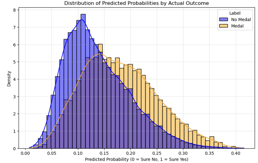
Solution:
Apply “Weights” to the Loss Function (Weighted Loss) Modify the JAX/Optax code slightly to increase the penalty for medal-winning data by about 10 to 15 times.
Then I asked to Gemini again to improve model.
import pandas as pd
import numpy as np
import jax
import jax.numpy as jnp
from flax import linen as nn
from flax.training import train_state
import optax
from sklearn.preprocessing import LabelEncoder, StandardScaler
from sklearn.model_selection import train_test_split
from sklearn.metrics import confusion_matrix
import matplotlib.pyplot as plt
import seaborn as sns

# ==========================================
# 1. Data Preprocessing
# ==========================================
print("Loading and preprocessing data...")

df = pd.read_csv('datasets/olympic_athlete_events.csv')
df['Target'] = df['Medal'].apply(lambda x: 0 if pd.isna(x) else 1)

cat_cols = ['Sex', 'NOC', 'Sport', 'Season']
for col in cat_cols:
    le = LabelEncoder()
    df[col] = le.fit_transform(df[col].astype(str))

num_cols = ['Age', 'Height', 'Weight']
df[num_cols] = df[num_cols].fillna(df[num_cols].mean())
scaler = StandardScaler()
df[num_cols] = scaler.fit_transform(df[num_cols])

X_cat = df[cat_cols].values.astype(int)
X_num = df[num_cols].values.astype(float)
y = df['Target'].values.astype(int)

X_cat_train, X_cat_test, X_num_train, X_num_test, y_train, y_test = train_test_split(
    X_cat, X_num, y, test_size=0.2, random_state=42
)

# ---------------------------------------------------------
# ### NOTE: MODIFICATION 1 - Calculate Class Weight
# We calculate how many times more negative samples exist compared to positive ones.
# This value (pos_weight) will be used to penalize the model more when it misses a medal.
# ---------------------------------------------------------
n_pos = y_train.sum()
n_neg = len(y_train) - n_pos
pos_weight = n_neg / n_pos
print(f"Positive Weight calculated: {pos_weight:.2f}")

vocab_sizes = [df[c].max() + 1 for c in cat_cols]

# ==========================================
# 2. Model Definition (No changes here)
# ==========================================
class OlympicModel(nn.Module):
    vocab_sizes: list
    emb_dim: int = 10

    @nn.compact
    def __call__(self, x_cat, x_num):
        embs = []
        for i, vocab_size in enumerate(self.vocab_sizes):
            emb = nn.Embed(num_embeddings=vocab_size, features=self.emb_dim, name=f'emb_{i}')(x_cat[:, i])
            embs.append(emb)
        x_emb = jnp.concatenate(embs, axis=1)
        x = jnp.concatenate([x_emb, x_num], axis=1)
        x = nn.Dense(features=64)(x)
        x = nn.relu(x)
        x = nn.Dense(features=32)(x)
        x = nn.relu(x)
        x = nn.Dense(features=1)(x)
        return x

# ==========================================
# 3. Training Step
# ==========================================
def create_train_state(rng, learning_rate, vocab_sizes, sample_cat, sample_num):
    model = OlympicModel(vocab_sizes=vocab_sizes)
    params = model.init(rng, sample_cat, sample_num)['params']
    tx = optax.adam(learning_rate)
    return train_state.TrainState.create(apply_fn=model.apply, params=params, tx=tx)

@jax.jit
def train_step(state, x_cat, x_num, y, pos_weight): # ### NOTE: Added 'pos_weight' argument
    def loss_fn(params):
        logits = state.apply_fn({'params': params}, x_cat, x_num)

        # Standard Binary Cross Entropy
        bce = optax.sigmoid_binary_cross_entropy(logits, y.reshape(-1, 1))

        # ---------------------------------------------------------
        # ### NOTE: MODIFICATION 2 - Apply Weighted Mask
        # We create a mask where:
        # - If label is 1 (Medal), weight = pos_weight (e.g., 6.0)
        # - If label is 0 (No Medal), weight = 1.0
        # ---------------------------------------------------------
        weight_mask = jnp.where(y.reshape(-1, 1) == 1, pos_weight, 1.0)

        # ### NOTE: Multiply the raw loss by the mask before averaging
        loss = (bce * weight_mask).mean()
        return loss

    loss, grads = jax.value_and_grad(loss_fn)(state.params)
    state = state.apply_gradients(grads=grads)
    return state, loss

@jax.jit
def predict_step(state, x_cat, x_num):
    logits = state.apply_fn({'params': state.params}, x_cat, x_num)
    return nn.sigmoid(logits)

# ==========================================
# 4. Training Loop
# ==========================================
print("Training started...")

rng = jax.random.PRNGKey(42)
learning_rate = 0.001
epochs = 100

state = create_train_state(rng, learning_rate, vocab_sizes, X_cat_train[:1], X_num_train[:1])

for epoch in range(epochs):
    # ---------------------------------------------------------
    # ### NOTE: MODIFICATION 3 - Pass 'pos_weight' to train_step
    # ---------------------------------------------------------
    state, loss = train_step(state, X_cat_train, X_num_train, y_train, pos_weight)

    if epoch % 10 == 0:
        print(f"Epoch {epoch}: Loss = {loss:.4f}")

print("Training finished.")

# ==========================================
# 5. Visualization (Standard)
# ==========================================
# (Code below is for visualization and remains mostly standard,
# aside from plotting the result of the new weighted model)

pred_probs = predict_step(state, X_cat_test, X_num_test)
pred_probs = np.array(pred_probs).flatten()

plt.figure(figsize=(10, 6))
res_df = pd.DataFrame({'Actual': y_test, 'Prob': pred_probs})
res_df['Label'] = res_df['Actual'].map({0: 'No Medal', 1: 'Medal'})

sns.histplot(
    data=res_df, x='Prob', hue='Label',
    bins=50, kde=True, stat="density", common_norm=False,
    palette={'No Medal': 'blue', 'Medal': 'orange'}, alpha=0.5
)
plt.title(f'Prediction Distribution (Weighted Loss, Weight={pos_weight:.1f})')
plt.xlabel('Predicted Probability')
plt.grid(True, alpha=0.3)
plt.show()

pred_labels = (pred_probs >= 0.5).astype(int)
cm = confusion_matrix(y_test, pred_labels)

plt.figure(figsize=(6, 5))
sns.heatmap(cm, annot=True, fmt='d', cmap='Blues',
            xticklabels=['Pred No', 'Pred Yes'],
            yticklabels=['Actual No', 'Actual Yes'])
plt.title('Confusion Matrix')
plt.show()
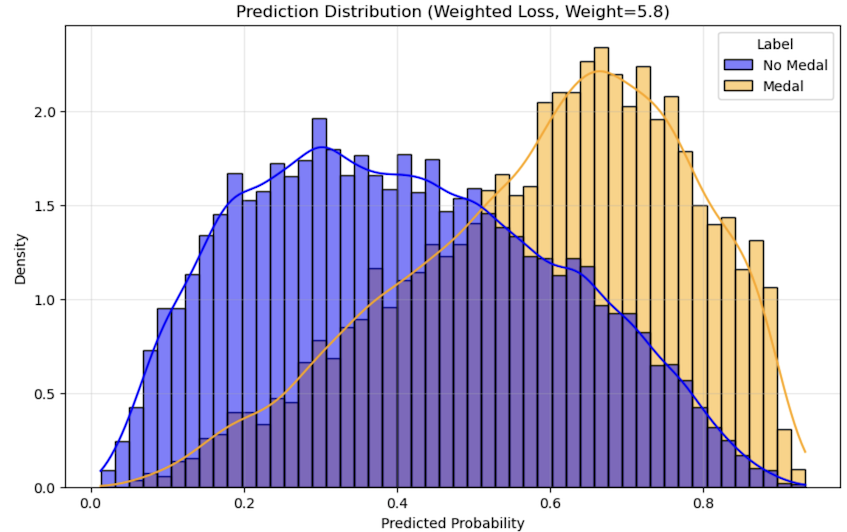
Loading and preprocessing data...
Positive Weight calculated: 5.81
Training started...
Epoch 0: Loss = 1.1889
Epoch 10: Loss = 1.1604
Epoch 20: Loss = 1.1431
Epoch 30: Loss = 1.1260
Epoch 40: Loss = 1.1080
Epoch 50: Loss = 1.0888
Epoch 60: Loss = 1.0696
Epoch 70: Loss = 1.0505
Epoch 80: Loss = 1.0322
Epoch 90: Loss = 1.0153
Training finished.


I could get the result! Let's analys this result.
Analysis①
The result getting better.
Firstly predicted probability got higher point. The model can predict medalist with over 0.5 point. It means the model caould predicted as a medalist for people who took medal with 50% probability.
Analysis②
Positive aspect (bottom right ④): Correctly identified 5,631 medalists!
Side effect (top right ②): However, it incorrectly predicted that 15,000 athletes could win medals (“You can win a medal too!”) (false positives).
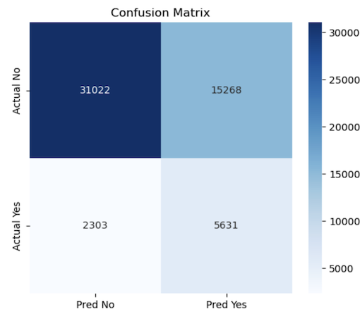
Conclusion
I could play with the data relate to olympic game medalists. Also I could try to make the prediction model using deep learning library called Jax. This library analyse the 54224 data in few minutes. Also I could improve the prediction model by changing the penalty adjustment.