Kae Nagano - Fab Futures - Data Science

Home About

Class

- Density Estimation

Assignment　　

• Fit a probability distribution to your data

Approach

1. K-means with Fab Academy Git data

As a first step, I referred to the class example and applied k-means clustering to explore the relationship between the total number of Git commits and the number of active weeks (weeks with at least one commit).

import matplotlib.pyplot as plt
from scipy.spatial import Voronoi,voronoi_plot_2d
import numpy as np
import time
import pandas as pd

# --- load data ---
df = pd.read_csv("datasets/fabacademy_commit_weekly_summary.csv")
week_cols = [c for c in df.columns if "week_" in c]
x = df["commit_total"].to_numpy()
y = (df[week_cols] > 0).sum(axis=1).to_numpy()



#
# k-means parameters
#
npts = 1000
nclusters = 3
nsteps = 10
xs = [0,5,10]
ys = [0,10,5]
np.random.seed(0)
#
# generate random data
#
#x = np.array([])
#y = np.array([])
'''for i in range(len(xs)):
    x = np.append(x,np.random.normal(loc=xs[i],scale=1,size=npts))
    y = np.append(y,np.random.normal(loc=ys[i],scale=1,size=npts))
    '''
#
# choose starting points
#
indices = np.random.uniform(low=0,high=len(x),size=nclusters).astype(int)
mux = x[indices]
muy = y[indices]
#
# plot before iteration
#
fig,ax = plt.subplots()
plt.plot(x,y,'.')
vor = Voronoi(np.stack((mux,muy),axis=1))
voronoi_plot_2d(vor,ax=ax,show_points=True,show_vertices=False,point_size=20)
plt.autoscale()
plt.title('before k-means iterations')
plt.show()
#
# do k-means iteration
#
for i in range(nsteps):
    #
    # find closest points
    #
    xm = np.outer(x,np.ones(len(mux)))
    ym = np.outer(y,np.ones(len(muy)))
    muxm = np.outer(np.ones(len(x)),mux)
    muym = np.outer(np.ones(len(x)),muy)
    distances = np.sqrt((xm-muxm)**2+(ym-muym)**2)
    mins = np.argmin(distances,axis=1)
    #
    # update means
    #
    for i in range(len(mux)):
        index = np.where(mins == i)
        mux[i] = np.sum(x[index])/len(index[0])
        muy[i] = np.sum(y[index])/len(index[0])
#
# plot after iteration
#
fig,ax = plt.subplots()
plt.plot(x,y,'.')
vor = Voronoi(np.stack((mux,muy),axis=1))
voronoi_plot_2d(vor,ax=ax,show_points=True,show_vertices=False,point_size=20)
plt.autoscale()
plt.title('after k-means iteration')
plt.show()

The clustering did not work as expected, so I asked ChatGPT and added standardization.

import matplotlib.pyplot as plt
from scipy.spatial import Voronoi, voronoi_plot_2d
import numpy as np
import pandas as pd
from sklearn.preprocessing import StandardScaler

# --- load data ---
df = pd.read_csv("datasets/fabacademy_commit_weekly_summary.csv")
week_cols = [c for c in df.columns if "week_" in c]

x_raw = df["commit_total"].to_numpy()
y_raw = (df[week_cols] > 0).sum(axis=1).to_numpy()

# --- normalize  ---
scaler = StandardScaler()
XY = np.vstack([x_raw, y_raw]).T
XY_scaled = scaler.fit_transform(XY)
x = XY_scaled[:,0]
y = XY_scaled[:,1]

# --- k-means parameters ---
nclusters = 3
nsteps = 15
np.random.seed(0)

# --- choose starting points ---
indices = np.random.choice(len(x), size=nclusters, replace=False)
mux = x[indices]
muy = y[indices]

# --- plot before ---
fig, ax = plt.subplots()
plt.plot(x, y, '.', alpha=0.5)
vor = Voronoi(np.stack((mux, muy), axis=1))
voronoi_plot_2d(vor, ax=ax, show_points=True, show_vertices=False, point_size=20)
plt.title("before k-means iteration")
plt.show()

# --- k-means iteration ---
for _ in range(nsteps):

    xm = np.outer(x, np.ones(len(mux)))
    ym = np.outer(y, np.ones(len(muy)))
    muxm = np.outer(np.ones(len(x)), mux)
    muym = np.outer(np.ones(len(x)), muy)

    distances = np.sqrt((xm - muxm)**2 + (ym - muym)**2)
    mins = np.argmin(distances, axis=1)

    for k in range(len(mux)):
        idx = np.where(mins == k)[0]
        if len(idx) > 0:
            mux[k] = np.mean(x[idx])
            muy[k] = np.mean(y[idx])

# --- plot after ---
fig, ax = plt.subplots()
plt.plot(x, y, '.', alpha=0.5)
vor = Voronoi(np.stack((mux, muy), axis=1))
voronoi_plot_2d(vor, ax=ax, show_points=True, show_vertices=False, point_size=20)
plt.title("after k-means iteration")
plt.show()

Observation:

2. Kernel Density Estimation

Gaussian mixture models　　

I also tried Gaussian Mixture Models using the total number of Git commits and the number of active weeks (weeks with at least one commit).

import matplotlib.pyplot as plt
from scipy.spatial import Voronoi,voronoi_plot_2d
import numpy as np
import time
#
# Gaussuam mixture model parameters
#
#npts = 3000
npts = 1509
nclusters = 3
nsteps = 25
nplot = 100
xs = [0,5,10]
ys = [0,10,5]
np.random.seed(0)
#
# generate random data
#
'''
x = np.array([])
y = np.array([])
for i in range(len(xs)):
    x = np.append(x,np.random.normal(loc=xs[i],scale=1,size=npts//nclusters))
    y = np.append(y,np.random.normal(loc=ys[i],scale=1,size=npts//nclusters))
'''

# --- load data ---
df = pd.read_csv("datasets/fabacademy_commit_weekly_summary.csv")
week_cols = [c for c in df.columns if "week_" in c]

x_raw = df["commit_total"].to_numpy()
y_raw = (df[week_cols] > 0).sum(axis=1).to_numpy()

# --- normalize (VERY IMPORTANT!) ---
scaler = StandardScaler()
XY = np.vstack([x_raw, y_raw]).T
XY_scaled = scaler.fit_transform(XY)
x = XY_scaled[:,0]
y = XY_scaled[:,1]



#
# choose starting points and initialize
#
indices = np.random.uniform(low=0,high=len(x),size=nclusters).astype(int)
mux = x[indices]
muy = y[indices]
varx = (np.max(x)-np.min(x))**2
vary = (np.max(y)-np.min(y))**2
pc = np.ones(nclusters)/nclusters
#
# plot before iteration
#
fig,ax = plt.subplots()
plt.plot(x,y,'.')
plt.errorbar(mux,muy,xerr=np.sqrt(varx),yerr=np.sqrt(vary),fmt='r.',markersize=20)
plt.autoscale()
plt.title('before iteration')
plt.show()
#
# do E-M iterations
#
for i in range(nsteps):
    #
    # construct matrices
    #
    xm = np.outer(x,np.ones(nclusters))
    ym = np.outer(y,np.ones(nclusters))
    muxm = np.outer(np.ones(npts),mux)
    muym = np.outer(np.ones(npts),muy)
    varxm = np.outer(np.ones(npts),varx)
    varym = np.outer(np.ones(npts),varx)
    pcm = np.outer(np.ones(npts),pc)
    #
    # use model to update probabilities
    #
    pvgc = (1/np.sqrt(2*np.pi*varxm))*\
       np.exp(-(xm-muxm)**2/(2*varxm))*\
       (1/np.sqrt(2*np.pi*varym))*\
       np.exp(-(ym-muym)**2/(2*varym))
    pvc = pvgc*np.outer(np.ones(npts),pc)
    pcgv = pvc/np.outer(np.sum(pvc,1),np.ones(nclusters))
    #
    # use probabilities to update model
    #
    pc = np.sum(pcgv,0)/npts
    mux = np.sum(xm*pcgv,0)/(npts*pc)
    muy = np.sum(ym*pcgv,0)/(npts*pc)
    varx = 0.1+np.sum((xm-muxm)**2*pcgv,0)/(npts*pc)
    vary = 0.1+np.sum((ym-muym)**2*pcgv,0)/(npts*pc)
#
# plot after iteration
#
fig,ax = plt.subplots()
plt.plot(x,y,'.')
plt.errorbar(mux,muy,xerr=np.sqrt(varx),yerr=np.sqrt(vary),fmt='r.',markersize=20)
plt.autoscale()
plt.title('after iteration')
plt.show()
#
# plot distribution
#
xplot = np.linspace(np.min(x),np.max(x),nplot)
yplot = np.linspace(np.min(y),np.max(y),nplot)
(X,Y) = np.meshgrid(xplot,yplot)
p = np.zeros((nplot,nplot))
for c in range(nclusters):
    p += np.exp(-(X-mux[c])**2/(2*varx[c]))/np.sqrt(2*np.pi*varx[c])\
       *np.exp(-(Y-muy[c])**2/(2*vary[c]))/np.sqrt(2*np.pi*vary[c])\
       *pc[c]
fig, ax = plt.subplots(subplot_kw={"projection":"3d"})
ax.plot_surface(X,Y,p)
plt.title('probability distribution')
plt.show()

3. Cluster-Weighted Modeling　 with Fab Academy DAta

also called mixture of experts, Bayesian networks, ... put functional models in Gaussian kernels can use covariances in low dimensions, variances in high dimensions

Using the total number of Git commits and the number of active weeks (weeks with at least one commit), I applied cluster-weighted modeling based on the class example.
For the labels, I used whether each student graduated (1) or did not graduate (0).

• Data Preparation
  • datasets/fabacademy_with_projects_direct_2019_2025.json

  {
      "year": 2019,
      "labs": [
        {
          "lab_name_raw": "AKGEC",
          "lab_name": "AKGEC",
          "lab_url": "https://fabacademy.org/2019/labs/akgec.html",
          "students": [
            {
              "name": "Rajat Ratewal",
              "url": "https://fabacademy.org/2019/labs/akgec/students/rajat-ratewal",
              "graduate_year": 2019,
              "project_match": {
                "count": 1,
                "projects": [
                  {
                    "id": 1286,
                    "path": "academany/fabacademy/2019/labs/akgec/students/rajat-ratewal",
                    "url": "https://gitlab.fabcloud.org/academany/fabacademy/2019/labs/akgec/students/rajat-ratewal"
                  }
                ]
              }
            },
  

import matplotlib.pyplot as plt
import numpy as np
from sklearn.preprocessing import StandardScaler
import pandas as pd
import json

#
# Fab Academy data preparation  ( add graduated label )
#
df = pd.read_csv("datasets/fabacademy_commit_weekly_summary.csv")

with open("datasets/fabacademy_with_projects_direct_2019_2025.json","r") as f:
    data = json.load(f)

records = []
for year in data:
    for lab in year["labs"]:
        for s in lab["students"]:
            graduated = 1 if s.get("graduate_year") is not None else 0
            pm = s.get("project_match", {})
            projects = pm.get("projects", [])
            for p in projects:
                pid = p.get("id", None)
                if pid is not None:
                    records.append({
                        "project_id": pid,
                        "graduated": graduated,
                    })

grad_df = pd.DataFrame(records)

df = df.merge(grad_df, on="project_id", how="left")
df["graduated"] = df["graduated"].fillna(0).astype(int)
print(df.head())

week_cols = [c for c in df.columns if "week_" in c]
x_raw = df["commit_total"].to_numpy()
y_raw = (df[week_cols] > 0).sum(axis=1).to_numpy()
state_raw = df["graduated"].astype(int).to_numpy()

samples = np.column_stack((x_raw, y_raw))  # shape: (npts, 2)
scaler = StandardScaler()
samples_scaled = scaler.fit_transform(samples)  # shape: (npts, 2)
points = samples_scaled.T  # shape: (2, npts)

states = state_raw
npts = len(states)


#
# state cluster-weighted modeling parameters
#
dim = 2
nstates = 2
nclusters = 5
momentum = 0.9
rate = 0.1
min_var = 0.1
niterations = 100
np.random.seed(10)

#
# initialize arrays
#
indices = np.random.randint(0,npts,nclusters)
means = points[:,indices]
dmean = np.zeros((dim,nclusters))
variances = np.outer(np.var(points,axis=1),np.ones(nclusters))
pc = np.ones(nclusters)/nclusters
pxgc = np.zeros((nclusters,npts))
psgxc = np.ones((nclusters,nstates))/nstates

print("=== INITIAL STATE ===")
print("initial means:\n", means)
print("initial variances:\n", variances)

#
# plot data
#
plt.plot(points[0,states==0],points[1,states==0],ls='',marker='$0$',markeredgecolor='green')
plt.plot(points[0,states==1],points[1,states==1],ls='',marker='$1$',markeredgecolor='orange')
plt.xlim([np.min(points[0,:])-1,np.max(points[0,:])+1])
plt.ylim([np.min(points[1,:])-1,np.max(points[1,:])+1])

#
# plot clusters
#
def plot_var():
   for cluster in range(means.shape[1]):
      x = means[0,cluster]
      y = means[1,cluster]
      type = np.argmax(psgxc[cluster,:])
      dx = np.sqrt(variances[0,cluster])
      dy = np.sqrt(variances[1,cluster])
      plt.plot([x-dx,x+dx],[y,y],'k')
      plt.plot([x,x],[y-dy,y+dy],'k')
      plt.plot([x],[y],'k',marker=f'${type}$',markersize=15)

plot_var()
plt.title('variance clusters before iteration')
plt.xlabel("Total Commits (standardized)")
plt.ylabel("Active Weeks (standardized)")
plt.show()

#
# do E-M iteration
#
for i in range(niterations):
   for cluster in range(nclusters):
      mean = np.outer(means[:,cluster],np.ones(npts))
      variance = np.outer(variances[:,cluster],np.ones(npts))
      pxgc[cluster,:] = np.prod(np.exp(-(points-mean)**2/(2*variance))\
         /np.sqrt(2*np.pi*variance),0)
   pxc = pxgc*np.outer(pc,np.ones(npts))
   pcgx = pxc/np.outer(np.ones(nclusters),np.sum(pxc,0))
   psxc = psgxc[:,states]*pxc
   pcgsx = psxc/np.outer(np.ones(nclusters),np.sum(psxc,0))
   pc = np.sum(pcgsx,1)/npts
   for cluster in range(nclusters):
      newmean = momentum*dmean[:,cluster]\
         +np.sum(points*np.outer(np.ones(dim),pcgsx[cluster,:]),1)\
         /np.sum(np.outer(np.ones(dim),pcgsx[cluster,:]),1)
      dmean[:,cluster] = newmean-means[:,cluster]
      means[:,cluster] += rate*dmean[:,cluster]
      m = np.outer(means[:,cluster],np.ones(npts))
      variances[:,cluster] = np.sum((points-m)**2\
          *np.outer(np.ones(dim),pcgsx[cluster,:]),1)\
         /np.sum(np.outer(np.ones(dim),pcgsx[cluster,:]),1)\
         +min_var
   for state in range(nstates):
      index = np.argwhere(states == state)
      psgxc[:,state] = np.sum(pcgsx[:,index],1)[:,0]/np.sum(pcgsx[:,:],1)
    
   if i % 20 == 0:
      print(f"\n=== iteration {i} ===")
      print("pcgsx (first 5 samples):\n", pcgsx[:, :5])
      print("means:\n", means)
      print("variances:\n", variances)
                                                         

#
# plot data
#
plt.plot(points[0,states==0],points[1,states==0],ls='',marker='$0$',markeredgecolor='green')
plt.plot(points[0,states==1],points[1,states==1],ls='',marker='$1$',markeredgecolor='orange')
plt.xlim([np.min(points[0,:])-1,np.max(points[0,:])+1])
plt.ylim([np.min(points[1,:])-1,np.max(points[1,:])+1])
plt.xlabel("Total Commits (standardized)")
plt.ylabel("Active Weeks (standardized)")
#
# plot clusters
#
plot_var()

#
# plot decision boundaries
#
ngrid = 100
xmin = np.min(points[0,:])
xmax = np.max(points[0,:])
ymin = np.min(points[1,:])
ymax = np.max(points[1,:])
x = np.linspace(xmin,xmax,ngrid)
y = np.linspace(ymin,ymax,ngrid)
mx,my = np.meshgrid(x,y)
x = np.reshape(mx,(ngrid*ngrid))
y = np.reshape(my,(ngrid*ngrid))
plotpoints = np.vstack((x,y))
pxgc = np.zeros((nclusters,ngrid*ngrid))
for cluster in range(nclusters):
   mean = np.outer(means[:,cluster],np.ones(ngrid*ngrid))
   variance = np.outer(variances[:,cluster],np.ones(ngrid*ngrid))
   pxgc[cluster,:] = np.prod(np.exp(-(plotpoints-mean)**2/(2*variance))\
      /np.sqrt(2*np.pi*variance),0)
pxc = pxgc*np.outer(pc,np.ones(ngrid*ngrid))
p = np.sum(np.outer(psgxc[:,1],np.ones(ngrid*ngrid))*pxc,0)/np.sum(pxc,0)
p = np.reshape(p,(ngrid,ngrid))
plt.contour(mx,my,p,[0.5])
plt.title('variance clusters and decision boundaries after iteration')

for k in range(nclusters):
    x, y = means[:, k]
    plt.text(x, y+0.2, f"{k}", color="red", fontsize=14, weight="bold")
plt.show()
    
#
# plot probability surface
#
fig, ax = plt.subplots(subplot_kw={"projection":"3d"})
ax.plot_wireframe(mx,my,p,rstride=10,cstride=10,color='gray')
plt.plot(points[0,states==0],points[1,states==0],zdir='z',ls='',marker='r$0$',markeredgecolor='green')
plt.plot(points[0,states==1],points[1,states==1],zdir='z',ls='',marker='$1$',markeredgecolor='orange')
plt.title('probability of graduating (state 1)')
ax.set_xlabel("Git Commit Count (std.)")
ax.set_ylabel("Active Weeks (std.)")
ax.set_zlabel("Graduation Probability")
plt.show()

#
# Cluster ID
#
cluster_ids = np.argmax(pcgsx, axis=0)
df["cluster_id"] = cluster_ids

print("\n=== FINAL CLUSTER ASSIGNMENT ===")
print("cluster counts:", np.bincount(cluster_ids))
print("cluster_ids (first 20):", cluster_ids[:20])
df.to_csv("datasets/fabacademy_commit_weekly_summary_with_cluster.csv", index=False)

   project_id  year lab_name     student_name  \
0        1286  2019    AKGEC    Rajat Ratewal   
1        1287  2019    AKGEC  Narender Sharma   
2        1285  2019    AKGEC   Ashish Sawhney   
3        1290  2019    AKGEC     Jay Dhariwal   
4        1289  2019    AKGEC        Ahmad Ali   

                                         student_url  commit_total  \
0  https://fabacademy.org/2019/labs/akgec/student...            93   
1  https://fabacademy.org/2019/labs/akgec/student...            76   
2  https://fabacademy.org/2019/labs/akgec/student...            60   
3  https://fabacademy.org/2019/labs/akgec/student...           436   
4  https://fabacademy.org/2019/labs/akgec/student...           178   

                    first_commit                    last_commit  week_01  \
0  2019-01-22T10:18:25.000+05:30  2019-06-18T20:57:24.000+05:30        5   
1  2019-01-26T16:09:32.000+00:00  2019-07-16T12:08:12.000+05:30        0   
2  2019-01-25T18:06:56.000+05:30  2019-04-30T17:34:07.000+05:30        0   
3  2019-01-23T17:21:47.000+05:30  2019-07-02T22:00:56.000+05:30        0   
4  2019-01-26T14:36:19.000+00:00  2019-07-07T21:10:13.000+05:30        0   

   week_02  ...  week_22  week_23  week_24  week_25  week_26  week_27  \
0       10  ...        7        0        0        0        0        0   
1       18  ...        6        7        2        1        1        0   
2       23  ...        0        0        0        0        0        0   
3       77  ...       16       17       16        0        0        0   
4        1  ...        1       25       28        7        0        0   

   week_28  week_29  week_30  graduated  
0        0        0        0          1  
1        0        0        0          1  
2        0        0        0          0  
3        0        0        0          1  
4        0        0        0          1  

[5 rows x 39 columns]
=== INITIAL STATE ===
initial means:
 [[-0.44120982 -0.04209935  2.42299473 -0.81214779 -0.45999149]
 [-1.74266354  0.05971063  0.31719266 -1.35644051 -1.48518152]]
initial variances:
 [[1. 1. 1. 1. 1.]
 [1. 1. 1. 1. 1.]]

=== iteration 0 ===
pcgsx (first 5 samples):
 [[0.04079797 0.05033586 0.24308139 0.00974343 0.04299364]
 [0.77075836 0.73037864 0.16762755 0.4414894  0.75524682]
 [0.01648586 0.01241336 0.00153853 0.51725384 0.04179885]
 [0.09538906 0.11534593 0.30009103 0.01317395 0.08248496]
 [0.07656876 0.09152621 0.2876615  0.01833937 0.07747573]]
means:
 [[-0.44076397 -0.04372788  2.37553325 -0.77505202 -0.45382571]
 [-1.65299083  0.10504431  0.36207465 -1.28443505 -1.40389911]]
variances:
 [[0.29797491 0.35295058 3.05468787 0.37603603 0.30795111]
 [1.38973813 0.77391162 0.71317675 1.27313915 1.36613791]]

=== iteration 20 ===
pcgsx (first 5 samples):
 [[9.93622984e-03 1.56008412e-02 3.26790850e-01 2.65028431e-05
  6.35586568e-03]
 [9.48306415e-01 9.25147994e-01 1.94210323e-03 9.29562478e-01
  9.61370638e-01]
 [7.32297031e-03 7.82204451e-03 1.13548027e-03 7.00722186e-02
  8.14192736e-03]
 [9.57095789e-03 1.49896368e-02 3.88020755e-01 2.10020944e-04
  7.68682550e-03]
 [2.48634273e-02 3.64394832e-02 2.82110811e-01 1.28780016e-04
  1.64447437e-02]]
means:
 [[-0.47343591  0.10091222  2.69152185 -0.42643434 -0.43834146]
 [-0.92524246  0.74094345  0.42541603 -0.87939927 -0.79420413]]
variances:
 [[0.20839976 0.39297959 2.974327   0.269635   0.21846114]
 [0.57613224 0.31829148 0.78406621 0.56693994 0.64787531]]

=== iteration 40 ===
pcgsx (first 5 samples):
 [[1.36924412e-03 2.92518286e-03 6.53033301e-01 3.97475015e-07
  8.11111430e-04]
 [9.66148412e-01 9.55508263e-01 9.03518007e-03 8.59325320e-01
  9.70867916e-01]
 [1.22208644e-02 1.23998713e-02 7.74823572e-04 1.40258942e-01
  1.28075350e-02]
 [5.82731701e-03 8.86534828e-03 2.14020536e-01 6.54856747e-05
  4.26722879e-03]
 [1.44341622e-02 2.03013345e-02 1.23136159e-01 3.49854678e-04
  1.12462084e-02]]
means:
 [[-0.59823116  0.04594098  2.46659585 -0.42661089 -0.36232738]
 [-1.15017195  0.66144447  0.61651391 -0.79073272 -0.66707915]]
variances:
 [[0.17685197 0.36885601 2.97803582 0.24333229 0.25598487]
 [0.38970964 0.38541323 0.6929043  0.56258358 0.62264021]]

=== iteration 60 ===
pcgsx (first 5 samples):
 [[1.18144761e-02 2.09450921e-02 9.70466558e-01 2.05073654e-05
  7.44422501e-03]
 [9.72823776e-01 9.62998828e-01 5.14761563e-03 8.16609928e-01
  9.76056671e-01]
 [1.16413635e-02 1.16609251e-02 3.07069598e-04 1.71205019e-01
  1.21851016e-02]
 [1.32928623e-03 1.60584768e-03 1.46216204e-02 3.83290537e-03
  1.53591801e-03]
 [2.39109782e-03 2.78930665e-03 9.45713631e-03 8.33164034e-03
  2.77808420e-03]]
means:
 [[-0.53401951  0.01300487  2.55603818  0.34185177  0.41109641]
 [-0.97283871  0.70326558  0.78067199 -0.12469499 -0.01338167]]
variances:
 [[0.19769407 0.33683996 3.03742072 0.71776242 0.72833942]
 [0.48684077 0.35285985 0.58780268 0.621719   0.63509663]]

=== iteration 80 ===
pcgsx (first 5 samples):
 [[1.68352015e-02 2.84780765e-02 9.93627967e-01 5.84040601e-05
  1.09315562e-02]
 [9.73684881e-01 9.62274282e-01 5.05111647e-03 7.83472279e-01
  9.77491896e-01]
 [7.48174218e-03 7.30483535e-03 8.13552473e-05 1.31758439e-01
  7.71718433e-03]
 [6.97687826e-04 6.85669599e-04 8.13540288e-04 2.59020771e-02
  1.34308619e-03]
 [1.30048744e-03 1.25713635e-03 4.26021138e-04 5.88088012e-02
  2.51627732e-03]]
means:
 [[-0.51720361  0.00905448  2.92206922  1.25091988  1.41814073]
 [-0.93785175  0.70400624  0.87989508  0.2236297   0.29428099]]
variances:
 [[0.20834095 0.32483881 3.30456293 0.68112743 0.73871137]
 [0.51465941 0.34962538 0.53566329 0.6791331  0.72125249]]

=== FINAL CLUSTER ASSIGNMENT ===
cluster counts: [849 983  57  53  61]
cluster_ids (first 20): [1 1 0 1 1 0 1 1 1 0 0 0 1 1 2 2 4 4 1 0]

fig, ax = plt.subplots(subplot_kw={"projection": "3d"}, figsize=(7,6))
fig.patch.set_facecolor("black")
ax.set_facecolor("black")

# --- Wireframe: 
ax.plot_wireframe(mx, my, p,
                  rstride=12, cstride=12,
                  color="#DDDDDD",     
                  linewidth=1.0,      
                  alpha=0.9)           
ax.scatter(points[0, states==0], points[1, states==0], 0,
           color="#7FFFD4", s=8, alpha=0.8)
ax.scatter(points[0, states==1], points[1, states==1], 0,
           color="#FFD580", s=8, alpha=0.8)

ax.set_xlabel("Git Commit Count (std.)", color="white")
ax.set_ylabel("Active Weeks (std.)", color="white")
ax.set_zlabel("Graduation Probability", color="white")
ax.tick_params(colors="white")

ax.xaxis.pane.set_facecolor((0,0,0,0))
ax.yaxis.pane.set_facecolor((0,0,0,0))
ax.zaxis.pane.set_facecolor((0,0,0,0))
ax.grid(False)
ax.view_init(elev=30, azim=-45)

plt.show()

Observations:

• The model reveals that consistent weekly activity is a stronger indicator of graduation than total commit volume.
• Interestingly, students with moderate commits but high active weeks show the highest graduation probability, while those with high commits but irregular activity do not.
• This suggests that persistence matters more than intensity.

• Memo

  • During the EM iterations, the values in pcgsx gradually change as the model refines the cluster assignments.　pcgsx[c, n] represents the probability that sample n belongs to cluster c.

  • For example, at iteration 80, the first sample has: [[1.68352015e-02 2.84780765e-02 9.93627967e-01 5.84040601e-05 1.09315562e-02]

    This means that among clusters 0–4, cluster 2 has the highest probability (0.9936). Therefore, the model considers sample 0 to belong most strongly to cluster 2.

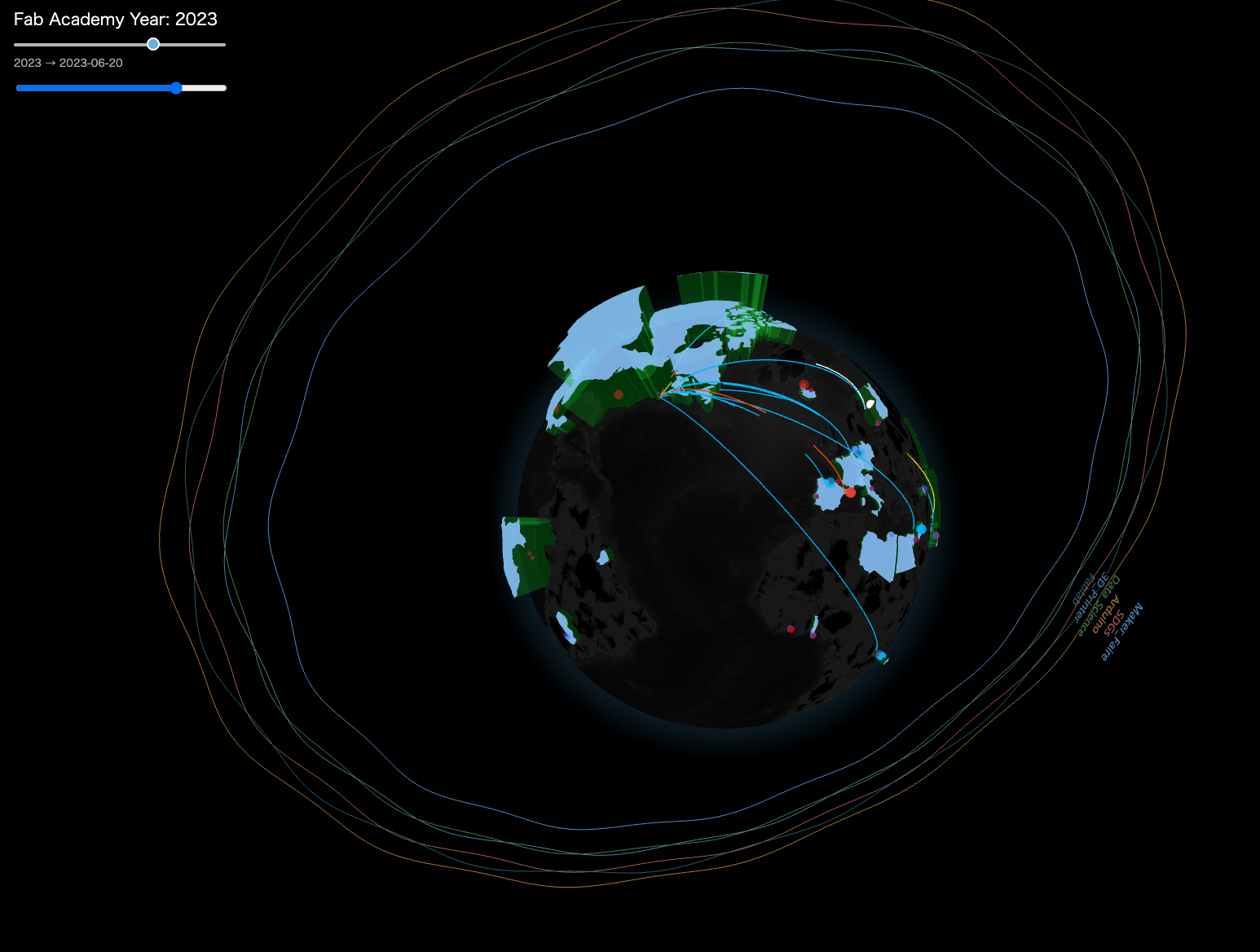
Commits Visualization

Building on the three.js globe I created in Week 1, I am now extending it to an interactive visualization that incorporates the clustering results.

Each commit is visualized as an arc drawn from the student’s lab to Boston (the assumed server location), using its timestamp. The color of the arc represents the cluster assigned to that student’s commit pattern.

Cluster0: Minimal Participants

Cluster1: Low Volume, Steady Progressors

Cluster2: High-Commit Burst Workers

Cluster3: Moderate, Consistent Contributors

Cluster4: High-Activity Multi-Taskers