FAB Futures - Data Science

Home About

Data Science/Session 4 > Machine Learning

Class Notes

Goals for the Week

• AI > emulate intelligence
• Machine Learning (ML) > use data to teach ML model
• Deep Learning (DL) > use Deep Neural Network model to learn from data

Neural Network

Neural Networks are modelled after the function of the human brain with neurons and perceptrons.

A single Input Layer with multiple Input Nodes feeds values into multiple Hidden Layers. Each Hidden Layer has multiple nodes and all of them receive all inputs from the Input Layer nodes or from all nodes of the preceding Hidden Layer. Each connection between nodes is qualified with significance weights and each Hidden Layer node is triggered based on specific Activation Functions (thresholds). The last Hidden Layer feeds into a fixed number of Output Nodes, with each node corresponding to all the possible outcomes being solved for by the model.

*image from Neil Gershenfeld's teaching notes*

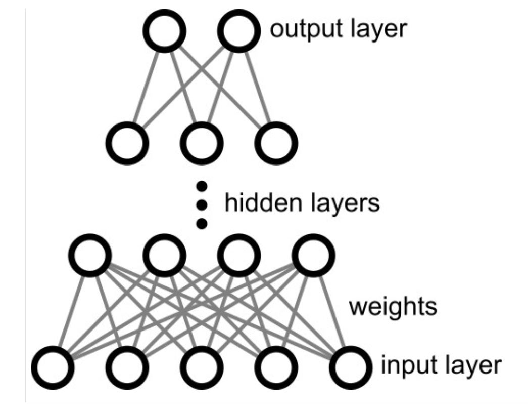
From what I could understand, the power of the Neural Network model as an outcome prediction tool is that it is Non-Linear in its decision making process (applying "non-linear activation functions"). The way the model is structured, with cross-linked nodes as pictured in the image above.

From Neil's notes, the following was written..."Exponential expressive power of network depth vs breadth". I asked ChatGPT for an explanation and received the following: "This phrase appears often in deep learning theory. It describes why deeper neural networks can represent certain functions MUCH more efficiently than wide, shallow networks." I am confused by the use of the words "expressive", "breadth",. "width", "deep" and "shallow" in this context, so I asked for further clarity. ChatGPT offered the following definitions:

• Expressive = the ability to model more complex shapes, more combination of features, more nonlinear problems
• Breadth = width and means many Neurons (previously described as nodes) in a single layer, but fewer layers...would try to solve everything in one huge step
• Depth = many layers (each with maybe fewer neurons)...would try to solve the problem with many (culmulative) smaller steps...and gives "exponential expressive power" to a model
• Deep vs Shallow...a deep network with a small number of neurons, but a shallow network would need an exponentially large number of neurons

Thus Neural Networks are deep and expressive.

Other terms defined by ChatGPT:

Activation Function = turns a neuron's linear output into a non-linear signal, giving a neural network the power to learn complex patterns. A small mathematical function applied to every neuron in a Neural Network...taking the neuron's input and decides what the neuron outputs. This 'decision' ability distinguishes it from a normal linear equation and allows Neural Networks to 'learn'. Activation functions introduce 'non-linearity'. Real world data (speech, images, handwriting, etc.) is non-linear.

Each neuron computes > z = weights * input + bias
...then the Activation Function is calculated > a = sigma_function * z

ReLU (if output negative, assign zero, otherwise assign one) is the most common activation function. Other activation functions include Sigmoid (good for binary classification), Tanh (good for positive and negative outcomes), and Softmax (vector into a probability, good for multi-class (multiple possible outcome) classification).

Loss Function = measures how wrong the model's predictions are. Compares the prediction with the correct answer. Returns an error value that should be minimized. Used in training a Neural Network model...to make it more effective.

Training

Neil goes through a huge list of concepts and terminology to explain Neural Network model training. The ones that stuck with me as very important include:

• Back Propagation = feeding back errors into the model to adjust and improve neuron weights...and hopefully prediction accuracy
• Gradient Descent = a specific mathematical procedure to reduce loss or errors
• Learning Rate = now small the adjustments made during gradient descent are
• Stochastic Gradient Descent = doing GD on a small subset of the big data set to increase speed and reduce memory demands

Models

Models can be built from scratch or be modified from existing ones available on Hugging Face, Kaggle, etc.

Frameworks

Python extensions to help with Machine Learning models include scikit-learn, JAX, PyTorch, and TensorFlow.

Research > Machine Learning

Dissecting Neils Code

Assignment

Python & Machine Learning

I found this tutorial series on YouTube that is similar to Neil's example from class.

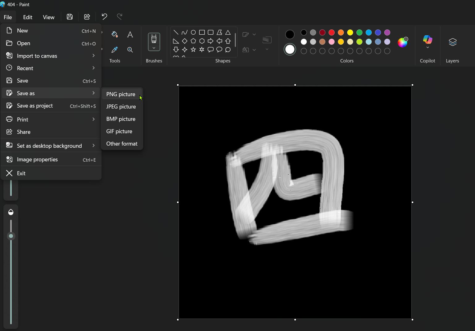
• Use MS Paint to generate characters for recognition. The video recommends the use of a "black" background (use the 'fill' tool) and the "oil brush".

In the 2nd Tutorial Video we are taught how to collect images from MS Paint. The procedure involves four steps:

1. Screen Capture
2. Generate dataset and load it
3. Fit the model using SVC and calculate accuracy
4. Prediction of image drawn in paint

Screen Capture

Two libraries are needed to make screen capture possible using Python code, 'pyscreenshot' and 'time'. The second library seems to already be part of my Python install. The first library requires a 'PIP install'.

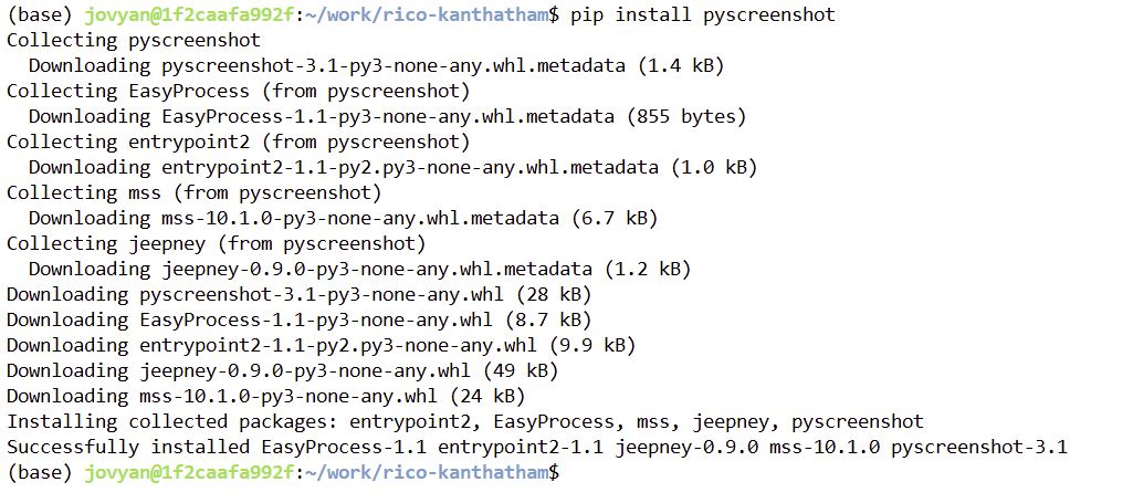
! pip install pyscreenshot

! pip install Pillow

! pip install mss

! pip install pyautogui

! pip install wxPython

# Screen Capture

# Needed Libraries
import pyscreenshot as ImageGrab
import time

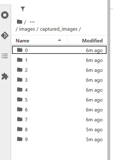
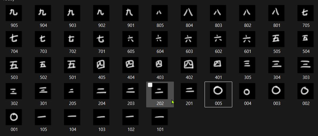
Folders need to be created to store screen capture images for characters to be recognized. A "captured_imaages" folder is created inside my "images" directory. Inside the "captured_images" folder, the tutorial says that individual folders for each character to be recognized should be created. I created a folder for each number from zero to nine.

Then in the code, the path to one of the character folders is specified and assigned to the variable "images_folder" followed by a For-Loop to capture 5 images every 8 seconds.

# 
images_folder = "images/auto_images/0/"
for i in range(0,5): #5 images
    time.sleep(8) # 8s interval
    im = ImageGrab.grab(bbox=(100,360,1000,1100)) #location of top left of pc window...adjust as required
    print("saved.....", i)
    im.save(images_folder+str(i)+'.png')
    print("clear screen and redraw now...")

saved..... 0

---------------------------------------------------------------------------
FileNotFoundError                         Traceback (most recent call last)
Cell In[8], line 7
      5 im = ImageGrab.grab(bbox=(100,360,1000,1100)) #location of top left of pc window...adjust as required
      6 print("saved.....", i)
----> 7 im.save(images_folder+str(i)+'.png')
      8 print("clear screen and redraw now...")

File c:\Users\senna\AppData\Local\Programs\Python\Python313\Lib\site-packages\PIL\Image.py:2566, in Image.save(self, fp, format, **params)
   2564         fp = builtins.open(filename, "r+b")
   2565     else:
-> 2566         fp = builtins.open(filename, "w+b")
   2567 else:
   2568     fp = cast(IO[bytes], fp)

FileNotFoundError: [Errno 2] No such file or directory: 'images/auto_images/0/0.png'

Well, dang it. The code generates an error. I ask ChatGPT for an explanation for the error and the upshot is...if I am running Jupyter Notebook on a Remote Server (I am)...the program CANNOT see my PC screen and screen capture is not possible.

So much for the cool technique to have screenshots automatically recorded into my Jupyter Notebook folder. I will have to take screen shots by hand and just add them to my folders manually.

Good to know that if I run Jupyter Notebook locally, I can do screenshots! Maybe this is a good time for me to try to figure out how to run my Jupyter Notebook locally on VScode? Or is this a time sink?
The Tutorial Part 3.

Training Data Generation

So I had to resort to drawing and saving characters (numbers 0 to 9) by hand in MS Paint. It didn't take that much time and it was kind of relaxing. I generated 5 versions of each number as it was done in the tutorial. I saved the 5 images for each number into their respectively named folder in my Jupyter Notebook.

Since the Machine Learning process will be an image recognition exercise, it occurred to me that it is not neccessary to use Roman Numerals. Any graphical shape with explicit numerical meaning will do. So I decided to use Japanese Numerals.

The Automated Screen Capture code is turned into a function, in case I can figure out how to get my Jupyter Notebook to be locallized in VScode.

# Automated Screen Capture Function  

def screen_capture():
    import pyscreenshot as ImageGrab
    import time
    
    images_folder = "images/captured_images/0/"
    for i in range(0,5): #5 images
        time.sleep(8) # 8s interval
        im = ImageGrab.grab(bbox=(60,170,400,500)) #location of top left of pc window...adjust as required
        print("saved.....", i)
        im.save(images_folder+str(i)+'.png')
        print("clear screen and redraw now...")

Generate Dataset from Character Images

The tutorial recommends installing 'opencv-python', 'scikit-learn' and 'pandas'. 'Pandas' is already installed, so as before, I pip install 'opencv-python' and 'scikit-learn'.

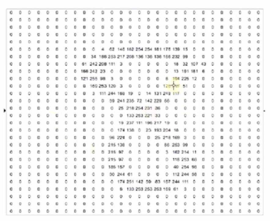
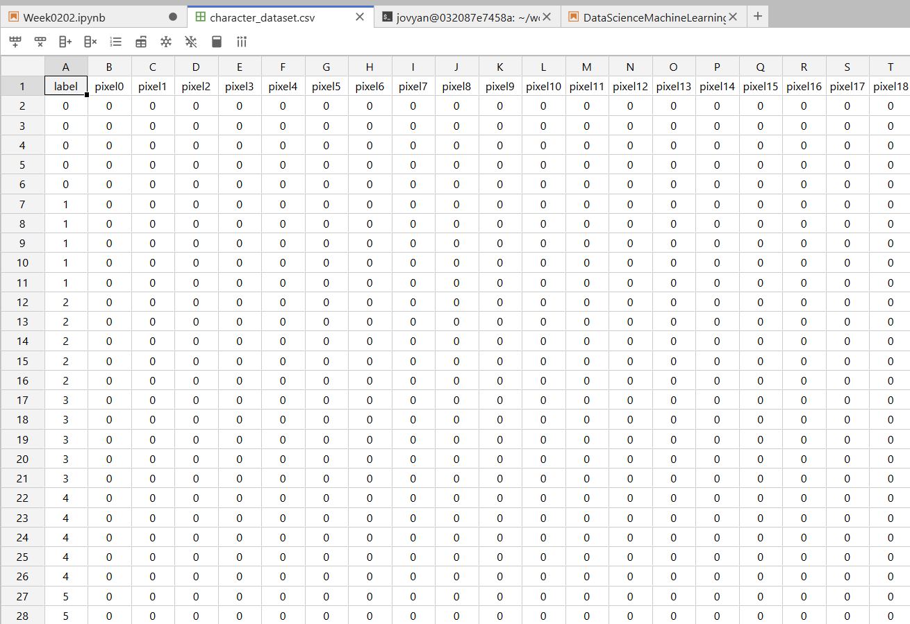
Now we move on to generate a dataset from the 200 images of the characters. The objective is to create a dataframe (a spreadsheet) 785 cells wide by 201 cells tall to contain image data for each number character image each with 784 pixels of color data. Each cell in the 28 x 28 matrix would be filled with a value representing a color in the greyscale range. A 'black' color would be assigned the lowest value zero, while a 'white' color would be assigned the highest value 255.

To build the dataframe the tutorial uses the following code, to which I made small modifications...

! pip install opencv-python

# Generate Dataset

import cv2
import csv
import glob

header = ["label"]
for i in range(0,784): #784 because a 28 x 28 matrix is being created
    header.append("pixel"+str(i)) # add extra header labels along the top of the dataframe
with open('datasets/character_dataset.csv', 'a') as f: #open a file, assign name "character_dataset.csv". "a" is append mode. Assign the file object to variablel "f"
    writer = csv.writer(f) #create CSV writer object that writes file f
    writer.writerow(header) #write a single row of header labels to CSV file
for label in range(10): #from 10 folders
    dirList = glob.glob("images/captured_images/"+str(label)+"/*.png")

    for img_path in dirList:
        im = cv2.imread(img_path) #read image data
        im_gray = cv2.cvtColor(im, cv2.COLOR_BGR2GRAY) #convert images to grey scale from BGR
        im_gray = cv2.GaussianBlur(im_gray,(15,15),0) #blur images with GaussianBlur to increase smoothness. 15,15 is kernel size. 0 is auto-calc sigma_x and sigma_y req'd to blur image.
        roi = cv2.resize(im_gray, (28,28), interpolation=cv2.INTER_AREA) #resize images to 28px x 28px. pass thru 1 method of interpolation. stored in variable 'roi' = region of interest
    
        data = []
        data.append(label)
        rows, cols = roi.shape

        # Add px one by one into data array
        for i in range(rows):
            for j in range(cols):
                k = roi[i,j]
                if k > 100: #k is greyscale value. zero is white. setting threshold at 100.
                    k = 1 #flatten data to 1 (black) or
                else:
                    k = 0 #...zero (white)
                data.append(k)
        with open('datasets/character_dataset.csv', 'a') as f: #Opens file in append mode
            writer = csv.writer(f) 
            writer.writerow(data) # Writes one row per processed image
    

The codes successfully creates a dataframe and saves it into the 'dataset' folder called "character_dataset.csv". Each row contains the data for one image, all 784 pixels. The number of Rows should equal the number of images. The number of columns equals the number of datapoints per character image. In my case, with 320 character images, I have a dataframe with 321 rows and 784 columns.

Loading the Dataset

With the dataframe built, the next step is to prepare the dataset for machine learning testing by shuffling the data rows. Scikit-learn's shuffle utility is used.

The tutorial's code is as follows...

! pip install pandas

! pip install scikit-learn

# Load Dataset  

import pandas as pd
from sklearn.utils import shuffle  #shuffle to randomly order data instead of ordered from small to large

data = pd.read_csv("datasets/character_dataset.csv")
data = shuffle(data)
data

	label	pixel0	pixel1	pixel2	pixel3	pixel4	pixel5	pixel6	pixel7	pixel8	...	pixel774	pixel775	pixel776	pixel777	pixel778	pixel779	pixel780	pixel781	pixel782	pixel783
308	9	0	0	0	0	0	0	0	0	0	...	0	0	0	0	0	0	0	0	0	0
196	6	0	0	0	0	0	0	0	0	0	...	0	0	0	0	0	0	0	0	0	0
12	0	0	0	0	0	0	0	0	0	0	...	0	0	0	0	0	0	0	0	0	0
63	1	0	0	0	0	0	0	0	0	0	...	0	0	0	0	0	0	0	0	0	0
309	9	0	0	0	0	0	0	0	0	0	...	0	0	0	0	0	0	0	0	0	0
...	...	...	...	...	...	...	...	...	...	...	...	...	...	...	...	...	...	...	...	...	...
217	6	0	0	0	0	0	0	0	0	0	...	0	0	0	0	0	0	0	0	0	0
139	4	0	0	0	0	0	0	0	0	0	...	0	0	0	0	0	0	0	0	0	0
31	0	0	0	0	0	0	0	0	0	0	...	0	0	0	0	0	0	0	0	0	0
173	5	0	0	0	0	0	0	0	0	0	...	0	0	0	0	0	0	0	0	0	0
152	4	0	0	0	0	0	0	0	0	0	...	0	0	0	0	0	0	0	0	0	0

320 rows × 785 columns

Row shuffling successfully completed.

Train the Model

The tutorial Part 3 suggests to install matplotlib and joblib python extensions using pip. I open the terminal and ran the commands, to discover that they are both already installed.

The next step, separate dependent and independent variables from the data. Remove the first column and assign the rest to the variable x. Assign rows to the variable y.

x = data.drop("label", axis= 1) #remove the 1st column from the dataframe. "1" causes vertical separation
y = data["label"]

Then, we test visualize one row of data (the data for a single image), selecting it by its index value, but reshape it frome a single row into a 28 x 28 pixel square. Use matplotlib to plot the image.

! pip install matplotlib

# preview one image using Matplotlib

%matplotlib inline
import matplotlib.pyplot as plt
import cv2
idx =  319 #input a row index value...from the 1st column
img = x.loc[idx].values.reshape(28,28) #grab x-values for the index row and reshape into a 28 x 28
print(y[idx])
plt.imshow(img)

9

<matplotlib.image.AxesImage at 0xe13a59a17d90>

Success!! the had drawn images are turned into a high-contrast, pixelized image. What was black is now purple. What was white is now yellow. Index 309 in the example is data for the number 9.

Separating into Training & Testing Data

• 20% of the available image data will be used for testing purposes
• 80% of the images are used for training purposes (more images should always be given for training purposes)
• Training images are used to create the model
• Testing images are used to calculate accuracy

Training: give both pixel value and label to the model. Must teach model. Provide pixel values and the label of those pixel values.

Testing: give only pixel values to the trained model, and ask it to return the label value. "Accuracy" is implied by the percentage of correct labels returned by the model.

# Test-Train Split

from sklearn.model_selection import train_test_split
train_x, test_x, train_y, test_y = train_test_split(x,y, test_size = 0.2) #0.2 = 20% of dataset images will be used for testing purposes

Fit a SVM Neural Network Model using SVC and Save the Model using Joblib

SVM is "Support vector machines (SVMs) are a set of supervised learning methods used for classification, regression and outliers detection." according to scikit-learn.org

SVC is "C-Support Vector Classification". Based on libsvm. "The fit time scales at least quadratically with the number of samples and may be impractical beyond tens of thousands of samples." The definition is from {Scikit-learn.org](https://scikit-learn.org/stable/modules/generated/sklearn.svm.SVC.html)

The following code from the tutorial creates a model with a fit function and saves it into the "model" folder. The SVC command is given "linear" kernel type and "random state" of 6.

kernel = "A kernel is the core part of an operating system. It acts as a bridge between software applications and the hardware of a computer." according to geeksforgeeks.org

import joblib
from sklearn.svm import SVC
classifier = SVC(kernel="linear", random_state=6) #
classifier.fit(train_x, train_y) #create model
joblib.dump(classifier, "model/digit_recognizer") #save model

['model/digit_recognizer']

Success!!

Calculate Accuracy

Use the metrics utility of Scikit-Learn to run accuracy calculations for the model.

from sklearn import metrics
predictions = classifier.predict(test_x) #using only x values, no need for y labels
print("Accuracy:  ", metrics.accuracy_score(predictions, test_y)) #accuracy_score compares the model predictions with the data value label

Accuracy:   0.9375

With the initial dataset of 50 character images, my model has an 80% accuracy at recognizing the number being suggested by the graphic. Not great. I think I still need more samples.

Update 1: Dataset Size Increased to 200 image samples, model accuracy increases to 85%.

Update 2 Dataset Size Increased by 120 samples, now 320 total. And model accuracy has improved to 93.75%

Extra Work: Running Jupyter Notebook Locally

I really wanted to run the above ML model locally, since the tutorial was suggesting that it could see what I was drawing on my Paint program and then make predictions real time. When I was running the code in remote server interface of Jupyter Notebook, the program could not see my Windows desktop. To have the program utilize its full functionality, I need to run Jupyter Notebook locally in VScode.

Long story short, it took some doing, but now I am able to update my documentation locally in VScode and push to the server via git. It also seems that I can run Python code locally. The process took lots of effort and help from ChatGPT. In brief, I needed to:

• clone my repository from Gitlab (using SSH)
• create an SSH key on my PC and add the public key to Gitlab
• install the Jupyter extension in VScode
• install the Python extension in VScode
• create a Python virtual environment in VScode
• install ipykernel

Now to test the program...

Had to:

• update a dependency for pyscreenshot with Pillow, compatible with the newest Python version

Modifying the Screen Capture code...

# Screen Capture

# Needed Libraries
import pyscreenshot as ImageGrab
import time

images_folder = "images/auto_images/94"
for i in range(0,10): #10 images
    time.sleep(8) # 8s interval
    im = ImageGrab.grab(bbox=(150,230,900,900)) #location of top left of pc window...adjust X1, Y1, X2, Y2 as required
    print("saved.....", i)
    im.save(images_folder+str(i)+'.png')
    print("clear screen and redraw now...")

OK! After a bit of tweaking, got the code to:

• capture images from the right place on the screen (where the drawing area of MS Paint is situated)
• write the name so that the last value of the code images_folder = "images/auto_images/0" is the prefix for the sequence of images that are shot and saved as PNG files.

The image data base has been increased to 500 data points (50 samples for each numerical digit from 0 to 9). Let's move on to generating a new ML model using the bigger dataset...and see if the Accuracy will improve!

Generate a Dataframe from the Dataset

! pip install Numpy

! pip install opencv-python

Dang it. OpenCV cannot be installed...because the latest version of Python does not have Numpy built in.

ChatGPT recommends > using an older (stable) version of Python, not the latest version (yet).

# Generate Dataset

import cv2
import csv
import glob

header = ["label"]
for i in range(0,784): 
    header.append("pixel"+str(i)) 
with open('datasets/character_dataset.csv', 'a') as f: #input correct dataset CSV file name
    writer = csv.writer(f) 
    writer.writerow(header) 
for label in range(10): 
    dirList = glob.glob("images/captured_images/"+str(label)+"/*.png") #specify the folder where training & testing images are stored
    for img_path in dirList:
        im = cv2.imread(img_path)
        im_gray = cv2.cvtColor(im, cv2.COLOR_BGR2GRAY) 
        im_gray = cv2.GaussianBlur(im_gray,(15,15),0) 
        roi = cv2.resize(im_gray, (28,28), interpolation=cv2.INTER_AREA)
    
        data = []
        data.append(label)
        rows, cols = roi.shape

        # Add px one by one into data array
        for i in range(rows):
            for j in range(cols):
                k = roi[i,j]
                if k > 100: #threshold value
                    k = 1 
                else:
                    k = 0
                data.append(k)
        with open('datasets/character_dataset.csv', 'a') as f: #Opens file in append mode
            writer = csv.writer(f) 
            writer.writerow(data) # Writes one row per processed image
    

Shuffle the Dataframe rows

# Load Dataset  

import pandas as pd
from sklearn.utils import shuffle  #shuffle to randomly order data instead of ordered from small to large

data = pd.read_csv("datasets/character_dataset.csv")
data = shuffle(data)
data

Separate Dependent/Independent Variables & Remove Label

x = data.drop("label", axis= 1) #remove the 1st column from the dataframe. "1" causes vertical separation
y = data["label"]

Preview Pixelated Image

# preview one image using Matplotlib

%matplotlib inline
import matplotlib.pyplot as plt
import cv2
idx =  319 #input a row index value...from the 1st column
img = x.loc[idx].values.reshape(28,28) #grab x-values for the index row and reshape into a 28 x 28
print(y[idx])
plt.imshow(img)

Split the Training Data > Training vs Testing

Test-Train Split

from sklearn.model_selection import train_test_split train_x, test_x, train_y, test_y = train_test_split(x,y, test_size = 0.2) #0.2 = 20% of dataset images will be used for testing purposes

Run SVM Neuro Network Fitting Function on Dataset

import joblib
from sklearn.svm import SVC
classifier = SVC(kernel="linear", random_state=6) #
classifier.fit(train_x, train_y) #create model
joblib.dump(classifier, "model/digit_recognizer") #save model

Calculate Model Accuracy

from sklearn import metrics
predictions = classifier.predict(test_x) #using only x values, no need for y labels
print("Accuracy:  ", metrics.accuracy_score(predictions, test_y)) #accuracy_score compares the model predictions with the data value label

(work incomplete...more to come)